
SLIDE 1
Another view
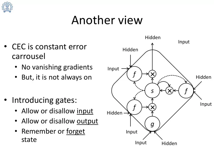
- CEC is constant error
carrousel
- No vanishing gradients
- But, it is not always on
- Introducing gates:
- Allow or disallow input
- Allow or disallow output
- Remember or forget
state
f g f s
× × ×
f
Input Hidden Input Hidden Hidden Hidden Input Input Input Hidden