Hidden Markov Models CMSC 473/673 UMBC Recap from last time - - PowerPoint PPT Presentation

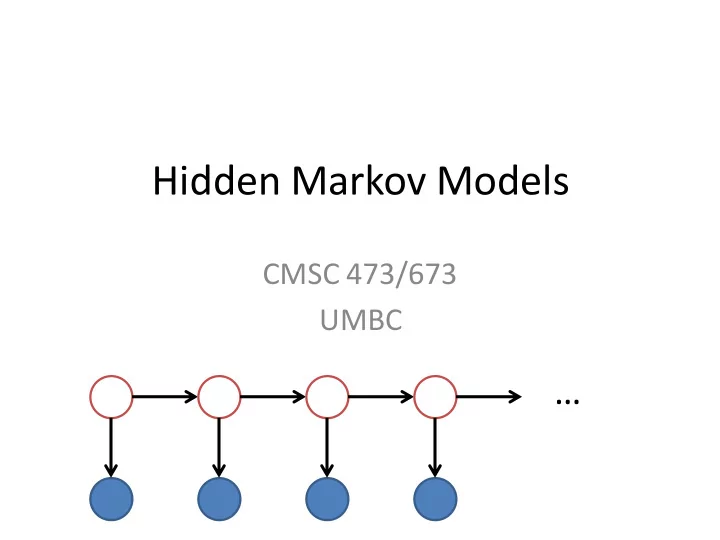
Hidden Markov Models

CMSC 473/673 UMBC

…

Recap from last time…

Expectation Maximization (EM)

• 0. Assume some value for your parameters

Two step, iterative algorithm

• 1. E-step: count under uncertainty, assuming these

parameters

• 2. M-step: maximize log-likelihood, assuming these

uncertain counts

estimated counts

Counting Requires Marginalizing

E-step: count under uncertainty, assuming these parameters

Counting Requires Marginalizing

w z1 & w z2 & w z3 & w z4 & w

E-step: count under uncertainty, assuming these parameters

break into 4 disjoint pieces

EM Example 1: Three Coins/Class-based Unigrams

Imagine three coins Flip 1st coin (penny) If heads: flip 2nd coin (dollar coin) If tails: flip 3rd coin (dime)

• bserved:

a, b, e, etc. We run the code, vs. The run failed unobserved: vowel or constonant? part of speech?

Outline

HMM Motivation (Part of Speech) and Brief Definition What is Part of Speech? HMM Detailed Definition HMM Tasks

Hidden Markov Models

Class-based Model

Use different distributions to explain groupings

• f observations

Sequence Model

Bigram model of the classes, not the

• bservations

Implicitly model all possible class sequences There exist algorithms for finding best sequence, and for the marginal likelihood

Hidden Markov Models: Part of Speech

p(British Left Waffles on Falkland Islands)

Adjective Noun Verb Noun Verb Noun Prep Noun Noun Prep Noun Noun (i): (ii):

Class-based model Bigram model

• f the classes

Model all class sequences

Hidden Markov Models: Part of Speech

p(British Left Waffles on Falkland Islands)

Adjective Noun Verb Noun Verb Noun Prep Noun Noun Prep Noun Noun (i): (ii):

Class-based model Bigram model

• f the classes

Model all class sequences

Hidden Markov Models: Part of Speech

p(British Left Waffles on Falkland Islands)

Adjective Noun Verb Noun Verb Noun Prep Noun Noun Prep Noun Noun (i): (ii):

Class-based model Bigram model

• f the classes

Model all class sequences

Hidden Markov Models: Part of Speech

p(British Left Waffles on Falkland Islands)

Adjective Noun Verb Noun Verb Noun Prep Noun Noun Prep Noun Noun (i): (ii):

Class-based model Bigram model

• f the classes

Model all class sequences

Hidden Markov Models: Part of Speech

p(British Left Waffles on Falkland Islands)

1. Explain this sentence as a sequence of (likely?) latent (unseen) tags (labels) 2. Produce a tag sequence for this sentence Adjective Noun Verb Noun Verb Noun Prep Noun Noun Prep Noun Noun (i): (ii):

Class-based model Bigram model

• f the classes

Model all class sequences

Agenda

HMM Motivation (Part of Speech) and Brief Definition What is Part of Speech? HMM Detailed Definition HMM Tasks

Parts of Speech

Classes of words that behave like one another in similar syntactic contexts Pronunciation (stress) can differ: object (noun: OB-ject) vs. object (verb: ob-JECT) It can help improve the inputs to other systems (text-to-speech, syntactic parsing)

Parts of Speech

Adapted from Luke Zettlemoyer

Nouns milk cat cats UMBC Baltimore bread speak give Verbs run Adjectives would-be wettest large happy red fake

Parts of Speech

Adapted from Luke Zettlemoyer

Nouns milk cat cats UMBC Baltimore bread speak give Verbs run Adjectives would-be wettest large happy red fake Determiners Conjunctions a the every what and

• r

if because Prepositions in under top

Parts of Speech

Adapted from Luke Zettlemoyer

Nouns milk cat cats UMBC Baltimore bread speak give Verbs run Adjectives would-be wettest large happy red fake can do may Determiners Conjunctions a the every what and

• r

if because Prepositions in under top

“I can eat.”

Parts of Speech

Adapted from Luke Zettlemoyer

Nouns milk cat cats UMBC Baltimore bread speak give Verbs run Adjectives would-be wettest large happy red fake can do may Determiners Conjunctions a the every what and

• r

if because Prepositions in under top

Parts of Speech

Adapted from Luke Zettlemoyer

Nouns milk cat cats UMBC Baltimore bread speak give Verbs run Adjectives would-be wettest large happy red fake can do may Determiners Conjunctions a the every what and

• r

if because Prepositions in under top Adverbs recently happily

Parts of Speech

Adapted from Luke Zettlemoyer

Nouns milk cat cats UMBC Baltimore bread speak give Verbs run Adjectives would-be wettest large happy red fake can do may Determiners Conjunctions a the every what and

• r

if because Prepositions in under top Adverbs recently happily

“Today, we eat there.”

then there (location)

Parts of Speech

Adapted from Luke Zettlemoyer

Nouns milk cat cats UMBC Baltimore bread speak give Verbs run Adjectives would-be wettest large happy red fake can do may Determiners Conjunctions a the every what and

• r

if because Prepositions in under top Adverbs recently happily

“I ate.” “There is a cat.”

then there (location) I you there

Parts of Speech

Adapted from Luke Zettlemoyer

Nouns milk cat cats UMBC Baltimore bread speak give Verbs run Adjectives would-be wettest large happy red fake can do may Determiners Conjunctions a the every what and

• r

if because Prepositions in under top Adverbs recently happily then there (location) I you there Numbers

• ne

1,324

Closed class words Open class words

Parts of Speech

Adapted from Luke Zettlemoyer

Nouns milk cat cats UMBC Baltimore bread speak give Verbs run Adjectives would-be wettest large happy red fake can do may Determiners Conjunctions a the every what and

• r

if because Prepositions in under top Adverbs recently happily then there (location) I you there Numbers

• ne

1,324

Parts of Speech

Adapted from Luke Zettlemoyer

Closed class words Open class words Nouns milk cat cats UMBC Baltimore bread speak give can do may Verbs Adjectives would-be wettest large happy red fake

Kamp & Partee (1995)

Adverbs recently happily then there (location)

intransitive

run

ditransitive transitive subsective non- subsective modals, auxiliaries

I you Determiners Prepositions Conjunctions

Pronouns

a the every what in under top and

• r

if because there Numbers

• ne

1,324

Parts of Speech

Adapted from Luke Zettlemoyer

Closed class words Open class words Nouns milk cat cats UMBC Baltimore bread speak give can do may Verbs Adjectives would-be wettest large happy red fake

Kamp & Partee (1995)

Adverbs recently happily then there (location)

intransitive

run

ditransitive transitive subsective non- subsective modals, auxiliaries

I you Determiners Prepositions Conjunctions

Pronouns

a the every what in under top Particles

(set) up

so (far) not (call)

• ff

and

• r

if because there Numbers

• ne

1,324

Parts of Speech

Adapted from Luke Zettlemoyer

Closed class words Open class words Nouns milk cat cats UMBC Baltimore bread speak give can do may Verbs Adjectives would-be wettest large happy red fake

Kamp & Partee (1995)

Adverbs recently happily then there (location)

intransitive

run

ditransitive transitive subsective non- subsective modals, auxiliaries

Numbers I you

• ne

1,324 Determiners Prepositions Conjunctions

Pronouns

and

• r

if a the every what in under top Particles

(set) up

so (far) not (call)

• ff

Language evolves! “I’m reading this because I want to procrastinate.” → “I’m reading this because procrastination.”

https://www.theatlantic.com/technology/archive/2013/11/english-has-a-new-preposition-because-internet/281601/

because because

Penn Treebank Part of Speech

3SLP: Chapter 10

http://universaldependencies.org/

Agenda

HMM Motivation (Part of Speech) and Brief Definition What is Part of Speech? HMM Detailed Definition HMM Tasks

Hidden Markov Models: Part of Speech

p(British Left Waffles on Falkland Islands)

Adjective Noun Verb Noun Verb Noun Prep Noun Noun Prep Noun Noun (i): (ii):

Class-based model Bigram model

• f the classes

Model all class sequences

𝑞 𝑥𝑗|𝑨𝑗

Hidden Markov Models: Part of Speech

p(British Left Waffles on Falkland Islands)

Adjective Noun Verb Noun Verb Noun Prep Noun Noun Prep Noun Noun (i): (ii):

Class-based model Bigram model

• f the classes

Model all class sequences

𝑞 𝑥𝑗|𝑨𝑗 𝑞 𝑨𝑗|𝑨𝑗−1

Hidden Markov Models: Part of Speech

p(British Left Waffles on Falkland Islands)

Adjective Noun Verb Noun Verb Noun Prep Noun Noun Prep Noun Noun (i): (ii):

Class-based model Bigram model

• f the classes

Model all class sequences

𝑞 𝑥𝑗|𝑨𝑗 𝑞 𝑨𝑗|𝑨𝑗−1

෍

𝑨1,..,𝑨𝑂

𝑞 𝑨1, 𝑥1, 𝑨2, 𝑥2, … , 𝑨𝑂, 𝑥𝑂

Hidden Markov Model

Goal: maximize (log-)likelihood In practice: we don’t actually observe these z values; we just see the words w

𝑞 𝑨1, 𝑥1, 𝑨2, 𝑥2, … , 𝑨𝑂, 𝑥𝑂 = 𝑞 𝑨1| 𝑨0 𝑞 𝑥1|𝑨1 ⋯ 𝑞 𝑨𝑂| 𝑨𝑂−1 𝑞 𝑥𝑂|𝑨𝑂 = ෑ

𝑗

𝑞 𝑥𝑗|𝑨𝑗 𝑞 𝑨𝑗| 𝑨𝑗−1

Hidden Markov Model

Goal: maximize (log-)likelihood In practice: we don’t actually observe these z values; we just see the words w

𝑞 𝑨1, 𝑥1, 𝑨2, 𝑥2, … , 𝑨𝑂, 𝑥𝑂 = 𝑞 𝑨1| 𝑨0 𝑞 𝑥1|𝑨1 ⋯ 𝑞 𝑨𝑂| 𝑨𝑂−1 𝑞 𝑥𝑂|𝑨𝑂 = ෑ

𝑗

𝑞 𝑥𝑗|𝑨𝑗 𝑞 𝑨𝑗| 𝑨𝑗−1

if we knew the probability parameters then we could estimate z and evaluate likelihood… but we don’t! :( if we did observe z, estimating the probability parameterswould be easy… but we don’t! :(

Hidden Markov Model Terminology

Each zi can take the value of one of K latent states

𝑞 𝑨1, 𝑥1, 𝑨2, 𝑥2, … , 𝑨𝑂, 𝑥𝑂 = 𝑞 𝑨1| 𝑨0 𝑞 𝑥1|𝑨1 ⋯ 𝑞 𝑨𝑂| 𝑨𝑂−1 𝑞 𝑥𝑂|𝑨𝑂 = ෑ

𝑗

𝑞 𝑥𝑗|𝑨𝑗 𝑞 𝑨𝑗| 𝑨𝑗−1

Hidden Markov Model Terminology

Each zi can take the value of one of K latent states

𝑞 𝑨1, 𝑥1, 𝑨2, 𝑥2, … , 𝑨𝑂, 𝑥𝑂 = 𝑞 𝑨1| 𝑨0 𝑞 𝑥1|𝑨1 ⋯ 𝑞 𝑨𝑂| 𝑨𝑂−1 𝑞 𝑥𝑂|𝑨𝑂 = ෑ

𝑗

𝑞 𝑥𝑗|𝑨𝑗 𝑞 𝑨𝑗| 𝑨𝑗−1

transition probabilities/parameters

Hidden Markov Model Terminology

Each zi can take the value of one of K latent states

𝑞 𝑨1, 𝑥1, 𝑨2, 𝑥2, … , 𝑨𝑂, 𝑥𝑂 = 𝑞 𝑨1| 𝑨0 𝑞 𝑥1|𝑨1 ⋯ 𝑞 𝑨𝑂| 𝑨𝑂−1 𝑞 𝑥𝑂|𝑨𝑂 = ෑ

𝑗

𝑞 𝑥𝑗|𝑨𝑗 𝑞 𝑨𝑗| 𝑨𝑗−1

emission probabilities/parameters transition probabilities/parameters

Hidden Markov Model Terminology

Each zi can take the value of one of K latent states Transition and emission distributions do not change

𝑞 𝑨1, 𝑥1, 𝑨2, 𝑥2, … , 𝑨𝑂, 𝑥𝑂 = 𝑞 𝑨1| 𝑨0 𝑞 𝑥1|𝑨1 ⋯ 𝑞 𝑨𝑂| 𝑨𝑂−1 𝑞 𝑥𝑂|𝑨𝑂 = ෑ

𝑗

𝑞 𝑥𝑗|𝑨𝑗 𝑞 𝑨𝑗| 𝑨𝑗−1

emission probabilities/parameters transition probabilities/parameters

Hidden Markov Model Terminology

Each zi can take the value of one of K latent states Transition and emission distributions do not change Q: How many different probability values are there with K states and V vocab items?

𝑞 𝑨1, 𝑥1, 𝑨2, 𝑥2, … , 𝑨𝑂, 𝑥𝑂 = 𝑞 𝑨1| 𝑨0 𝑞 𝑥1|𝑨1 ⋯ 𝑞 𝑨𝑂| 𝑨𝑂−1 𝑞 𝑥𝑂|𝑨𝑂 = ෑ

𝑗

𝑞 𝑥𝑗|𝑨𝑗 𝑞 𝑨𝑗| 𝑨𝑗−1

emission probabilities/parameters transition probabilities/parameters

Hidden Markov Model Terminology

Each zi can take the value of one of K latent states Transition and emission distributions do not change Q: How many different probability values are there with K states and V vocab items? A: VK emission values and K2 transition values

𝑞 𝑨1, 𝑥1, 𝑨2, 𝑥2, … , 𝑨𝑂, 𝑥𝑂 = 𝑞 𝑨1| 𝑨0 𝑞 𝑥1|𝑨1 ⋯ 𝑞 𝑨𝑂| 𝑨𝑂−1 𝑞 𝑥𝑂|𝑨𝑂 = ෑ

𝑗

𝑞 𝑥𝑗|𝑨𝑗 𝑞 𝑨𝑗| 𝑨𝑗−1

emission probabilities/parameters transition probabilities/parameters

Hidden Markov Model Representation

𝑞 𝑨1, 𝑥1, 𝑨2, 𝑥2, … , 𝑨𝑂, 𝑥𝑂 = 𝑞 𝑨1| 𝑨0 𝑞 𝑥1|𝑨1 ⋯ 𝑞 𝑨𝑂| 𝑨𝑂−1 𝑞 𝑥𝑂|𝑨𝑂 = ෑ

𝑗

𝑞 𝑥𝑗|𝑨𝑗 𝑞 𝑨𝑗| 𝑨𝑗−1

emission probabilities/parameters transition probabilities/parameters

z1

w1

…

w2 w3 w4

z2 z3 z4

represent the probabilities and independence assumptions in a graph

Hidden Markov Model Representation

𝑞 𝑨1, 𝑥1, 𝑨2, 𝑥2, … , 𝑨𝑂, 𝑥𝑂 = 𝑞 𝑨1| 𝑨0 𝑞 𝑥1|𝑨1 ⋯ 𝑞 𝑨𝑂| 𝑨𝑂−1 𝑞 𝑥𝑂|𝑨𝑂 = ෑ

𝑗

𝑞 𝑥𝑗|𝑨𝑗 𝑞 𝑨𝑗| 𝑨𝑗−1

emission probabilities/parameters transition probabilities/parameters

z1

w1

…

w2 w3 w4

z2 z3 z4

Graphical Models (see 478/678)

Hidden Markov Model Representation

𝑞 𝑨1, 𝑥1, 𝑨2, 𝑥2, … , 𝑨𝑂, 𝑥𝑂 = 𝑞 𝑨1| 𝑨0 𝑞 𝑥1|𝑨1 ⋯ 𝑞 𝑨𝑂| 𝑨𝑂−1 𝑞 𝑥𝑂|𝑨𝑂 = ෑ

𝑗

𝑞 𝑥𝑗|𝑨𝑗 𝑞 𝑨𝑗| 𝑨𝑗−1

emission probabilities/parameters transition probabilities/parameters

z1

w1

…

w2 w3 w4

z2 z3 z4

𝑞 𝑥1|𝑨1 𝑞 𝑥2|𝑨2 𝑞 𝑥3|𝑨3 𝑞 𝑥4|𝑨4

Hidden Markov Model Representation

𝑞 𝑨1, 𝑥1, 𝑨2, 𝑥2, … , 𝑨𝑂, 𝑥𝑂 = 𝑞 𝑨1| 𝑨0 𝑞 𝑥1|𝑨1 ⋯ 𝑞 𝑨𝑂| 𝑨𝑂−1 𝑞 𝑥𝑂|𝑨𝑂 = ෑ

𝑗

𝑞 𝑥𝑗|𝑨𝑗 𝑞 𝑨𝑗| 𝑨𝑗−1

emission probabilities/parameters transition probabilities/parameters

z1

w1

…

w2 w3 w4

z2 z3 z4

𝑞 𝑥1|𝑨1 𝑞 𝑥2|𝑨2 𝑞 𝑥3|𝑨3 𝑞 𝑥4|𝑨4

𝑞 𝑨2| 𝑨1 𝑞 𝑨3| 𝑨2 𝑞 𝑨4| 𝑨3

Hidden Markov Model Representation

𝑞 𝑨1, 𝑥1, 𝑨2, 𝑥2, … , 𝑨𝑂, 𝑥𝑂 = 𝑞 𝑨1| 𝑨0 𝑞 𝑥1|𝑨1 ⋯ 𝑞 𝑨𝑂| 𝑨𝑂−1 𝑞 𝑥𝑂|𝑨𝑂 = ෑ

𝑗

𝑞 𝑥𝑗|𝑨𝑗 𝑞 𝑨𝑗| 𝑨𝑗−1

emission probabilities/parameters transition probabilities/parameters

z1

w1

…

w2 w3 w4

z2 z3 z4

𝑞 𝑥1|𝑨1 𝑞 𝑥2|𝑨2 𝑞 𝑥3|𝑨3 𝑞 𝑥4|𝑨4

𝑞 𝑨2| 𝑨1 𝑞 𝑨3| 𝑨2 𝑞 𝑨4| 𝑨3 𝑞 𝑨1| 𝑨0 initial starting distribution (“BOS”)

Hidden Markov Model Representation

𝑞 𝑨1, 𝑥1, 𝑨2, 𝑥2, … , 𝑨𝑂, 𝑥𝑂 = 𝑞 𝑨1| 𝑨0 𝑞 𝑥1|𝑨1 ⋯ 𝑞 𝑨𝑂| 𝑨𝑂−1 𝑞 𝑥𝑂|𝑨𝑂 = ෑ

𝑗

𝑞 𝑥𝑗|𝑨𝑗 𝑞 𝑨𝑗| 𝑨𝑗−1

emission probabilities/parameters transition probabilities/parameters

z1

w1

…

w2 w3 w4

z2 z3 z4

𝑞 𝑥1|𝑨1 𝑞 𝑥2|𝑨2 𝑞 𝑥3|𝑨3 𝑞 𝑥4|𝑨4

𝑞 𝑨2| 𝑨1 𝑞 𝑨3| 𝑨2 𝑞 𝑨4| 𝑨3 𝑞 𝑨1| 𝑨0 initial starting distribution (“BOS”)

Each zi can take the value of one of K latent states Transition and emission distributions do not change

Example: 2-state Hidden Markov Model as a Lattice

z1 = N

w1

…

w2 w3 w4

z2 = N z3 = N z4 = N z1 = V z2 = V z3 = V z4 = V

…

Example: 2-state Hidden Markov Model as a Lattice

z1 = N

w1

…

w2 w3 w4

𝑞 𝑥1|𝑂 𝑞 𝑥2|𝑂 𝑞 𝑥3|𝑂 𝑞 𝑥4|𝑂

z2 = N z3 = N z4 = N z1 = V z2 = V z4 = V

…

𝑞 𝑥4|𝑊 𝑞 𝑥3|𝑊 𝑞 𝑥2|𝑊 𝑞 𝑥1|𝑊

z3 = V

Example: 2-state Hidden Markov Model as a Lattice

z1 = N

w1

…

w2 w3 w4

𝑞 𝑥1|𝑂 𝑞 𝑥2|𝑂 𝑞 𝑥3|𝑂 𝑞 𝑥4|𝑂

𝑞 𝑂| start z2 = N z3 = N z4 = N z1 = V z2 = V z3 = V z4 = V 𝑞 𝑊| 𝑊 𝑞 𝑊| 𝑊 𝑞 𝑊| 𝑊 𝑞 𝑊| start

…

𝑞 𝑥4|𝑊 𝑞 𝑥3|𝑊 𝑞 𝑥2|𝑊 𝑞 𝑥1|𝑊

𝑞 𝑂| 𝑂 𝑞 𝑂| 𝑂 𝑞 𝑂| 𝑂

Example: 2-state Hidden Markov Model as a Lattice

z1 = N

w1

…

w2 w3 w4

𝑞 𝑥1|𝑂 𝑞 𝑥2|𝑂 𝑞 𝑥3|𝑂 𝑞 𝑥4|𝑂

𝑞 𝑂| start z2 = N z3 = N z4 = N z1 = V z2 = V z3 = V z4 = V 𝑞 𝑊| 𝑊 𝑞 𝑊| 𝑊 𝑞 𝑊| 𝑊 𝑞 𝑊| start

…

𝑞 𝑊| 𝑂 𝑞 𝑊| 𝑂 𝑞 𝑊| 𝑂 𝑞 𝑂| 𝑊 𝑞 𝑂| 𝑊 𝑞 𝑂| 𝑊

𝑞 𝑥4|𝑊 𝑞 𝑥3|𝑊 𝑞 𝑥2|𝑊 𝑞 𝑥1|𝑊

𝑞 𝑂| 𝑂 𝑞 𝑂| 𝑂 𝑞 𝑂| 𝑂

Unigram Language Model

Comparison of Joint Probabilities

𝑞 𝑥1, 𝑥2, … , 𝑥𝑂 = 𝑞 𝑥1 𝑞 𝑥2 ⋯ 𝑞 𝑥𝑂 = ෑ

𝑗

𝑞 𝑥𝑗

Unigram Class-based Language Model (“K” coins) Unigram Language Model

Comparison of Joint Probabilities

𝑞 𝑥1, 𝑥2, … , 𝑥𝑂 = 𝑞 𝑥1 𝑞 𝑥2 ⋯ 𝑞 𝑥𝑂 = ෑ

𝑗

𝑞 𝑥𝑗 𝑞 𝑨1, 𝑥1, 𝑨2, 𝑥2, … ,𝑨𝑂, 𝑥𝑂 = 𝑞 𝑨1 𝑞 𝑥1|𝑨1 ⋯ 𝑞 𝑨𝑂 𝑞 𝑥𝑂|𝑨𝑂 = ෑ

𝑗

𝑞 𝑥𝑗|𝑨𝑗 𝑞 𝑨𝑗

Hidden Markov Model Unigram Class-based Language Model (“K” coins) Unigram Language Model

Comparison of Joint Probabilities

𝑞 𝑥1, 𝑥2, … , 𝑥𝑂 = 𝑞 𝑥1 𝑞 𝑥2 ⋯ 𝑞 𝑥𝑂 = ෑ

𝑗

𝑞 𝑥𝑗 𝑞 𝑨1, 𝑥1, 𝑨2, 𝑥2, … ,𝑨𝑂, 𝑥𝑂 = 𝑞 𝑨1 𝑞 𝑥1|𝑨1 ⋯ 𝑞 𝑨𝑂 𝑞 𝑥𝑂|𝑨𝑂 = ෑ

𝑗

𝑞 𝑥𝑗|𝑨𝑗 𝑞 𝑨𝑗 𝑞 𝑨1, 𝑥1, 𝑨2, 𝑥2, … , 𝑨𝑂, 𝑥𝑂 = 𝑞 𝑨1| 𝑨0 𝑞 𝑥1|𝑨1 ⋯ 𝑞 𝑨𝑂| 𝑨𝑂−1 𝑞 𝑥𝑂|𝑨𝑂 = ෑ

𝑗

𝑞 𝑥𝑗|𝑨𝑗 𝑞 𝑨𝑗| 𝑨𝑗−1

Estimating Parameters from Observed Data

z1 = N

w1 w2 w3 w4

𝑞 𝑥1|𝑂 𝑞 𝑥3|𝑂 𝑞 𝑥4|𝑂

𝑞 𝑂| start z2 = N z3 = N z4 = N z1 = V z2 = V z3 = V z4 = V 𝑞 𝑊| 𝑂 𝑞 𝑂| 𝑊

𝑞 𝑥2|𝑊

𝑞 𝑂| 𝑂 z1 = N

w1 w2 w3 w4

𝑞 𝑥1|𝑂 𝑞 𝑥4|𝑂

𝑞 𝑂| start z2 = N z3 = N z4 = N z1 = V z2 = V z3 = V z4 = V 𝑞 𝑊| 𝑊 𝑞 𝑊| 𝑂 𝑞 𝑂| 𝑊

𝑞 𝑥3|𝑊 𝑞 𝑥2|𝑊 N V end start N V w1 w2 W3 w4 N V Transition Counts Emission Counts

end emission not shown

Estimating Parameters from Observed Data

z1 = N

w1 w2 w3 w4

𝑞 𝑥1|𝑂 𝑞 𝑥3|𝑂 𝑞 𝑥4|𝑂

𝑞 𝑂| start z2 = N z3 = N z4 = N z1 = V z2 = V z3 = V z4 = V 𝑞 𝑊| 𝑂 𝑞 𝑂| 𝑊

𝑞 𝑥2|𝑊

𝑞 𝑂| 𝑂 z1 = N

w1 w2 w3 w4

𝑞 𝑥1|𝑂 𝑞 𝑥4|𝑂

𝑞 𝑂| start z2 = N z3 = N z4 = N z1 = V z2 = V z3 = V z4 = V 𝑞 𝑊| 𝑊 𝑞 𝑊| 𝑂 𝑞 𝑂| 𝑊

𝑞 𝑥3|𝑊 𝑞 𝑥2|𝑊 N V end start 2 N 1 2 2 V 2 1 w1 w2 W3 w4 N 2 1 2 V 2 1 Transition Counts Emission Counts

end emission not shown

Estimating Parameters from Observed Data

z1 = N

w1 w2 w3 w4

𝑞 𝑥1|𝑂 𝑞 𝑥3|𝑂 𝑞 𝑥4|𝑂

𝑞 𝑂| start z2 = N z3 = N z4 = N z1 = V z2 = V z3 = V z4 = V 𝑞 𝑊| 𝑂 𝑞 𝑂| 𝑊

𝑞 𝑥2|𝑊

𝑞 𝑂| 𝑂 z1 = N

w1 w2 w3 w4

𝑞 𝑥1|𝑂 𝑞 𝑥4|𝑂

𝑞 𝑂| start z2 = N z3 = N z4 = N z1 = V z2 = V z3 = V z4 = V 𝑞 𝑊| 𝑊 𝑞 𝑊| 𝑂 𝑞 𝑂| 𝑊

𝑞 𝑥3|𝑊 𝑞 𝑥2|𝑊 N V end start 1 N .2 .4 .4 V 2/3 1/3 w1 w2 W3 w4 N .4 .2 .4 V 2/3 1/3 Transition MLE Emission MLE

end emission not shown

Estimating Parameters from Observed Data

z1 = N

w1 w2 w3 w4

𝑞 𝑥1|𝑂 𝑞 𝑥3|𝑂 𝑞 𝑥4|𝑂

𝑞 𝑂| start z2 = N z3 = N z4 = N z1 = V z2 = V z3 = V z4 = V 𝑞 𝑊| 𝑂 𝑞 𝑂| 𝑊

𝑞 𝑥2|𝑊

𝑞 𝑂| 𝑂 z1 = N

w1 w2 w3 w4

𝑞 𝑥1|𝑂 𝑞 𝑥4|𝑂

𝑞 𝑂| start z2 = N z3 = N z4 = N z1 = V z2 = V z3 = V z4 = V 𝑞 𝑊| 𝑊 𝑞 𝑊| 𝑂 𝑞 𝑂| 𝑊

𝑞 𝑥3|𝑊 𝑞 𝑥2|𝑊 N V end start 1 N .2 .4 .4 V 2/3 1/3 w1 w2 W3 w4 N .4 .2 .4 V 2/3 1/3 Transition MLE Emission MLE

end emission not shown

smooth these values if needed

Outline

HMM Motivation (Part of Speech) and Brief Definition What is Part of Speech? HMM Detailed Definition HMM Tasks

Hidden Markov Model Tasks

Calculate the (log) likelihood of an observed sequence w1, …, wN Calculate the most likely sequence of states (for an

• bserved sequence)

Learn the emission and transition parameters

𝑞 𝑨1, 𝑥1, 𝑨2, 𝑥2, … , 𝑨𝑂, 𝑥𝑂 = 𝑞 𝑨1| 𝑨0 𝑞 𝑥1|𝑨1 ⋯ 𝑞 𝑨𝑂| 𝑨𝑂−1 𝑞 𝑥𝑂|𝑨𝑂 = ෑ

𝑗

𝑞 𝑥𝑗|𝑨𝑗 𝑞 𝑨𝑗| 𝑨𝑗−1

emission probabilities/parameters transition probabilities/parameters

Hidden Markov Model Tasks

Calculate the (log) likelihood of an observed sequence w1, …, wN Calculate the most likely sequence of states (for an

• bserved sequence)

Learn the emission and transition parameters

𝑞 𝑨1, 𝑥1, 𝑨2, 𝑥2, … , 𝑨𝑂, 𝑥𝑂 = 𝑞 𝑨1| 𝑨0 𝑞 𝑥1|𝑨1 ⋯ 𝑞 𝑨𝑂| 𝑨𝑂−1 𝑞 𝑥𝑂|𝑨𝑂 = ෑ

𝑗

𝑞 𝑥𝑗|𝑨𝑗 𝑞 𝑨𝑗| 𝑨𝑗−1

emission probabilities/parameters transition probabilities/parameters

HMM Likelihood Task

Marginalize over all latent sequence joint likelihoods

𝑞 𝑥1, 𝑥2, … , 𝑥𝑂 = ෍

𝑨1,⋯,𝑨𝑂

𝑞 𝑨1, 𝑥1, 𝑨2, 𝑥2, … , 𝑨𝑂, 𝑥𝑂

Q: In a K-state HMM for a length N observation sequence, how many summands (different latent sequences) are there?

HMM Likelihood Task

Marginalize over all latent sequence joint likelihoods

𝑞 𝑥1, 𝑥2, … , 𝑥𝑂 = ෍

𝑨1,⋯,𝑨𝑂

𝑞 𝑨1, 𝑥1, 𝑨2, 𝑥2, … , 𝑨𝑂, 𝑥𝑂

Q: In a K-state HMM for a length N observation sequence, how many summands (different latent sequences) are there? A: KN

HMM Likelihood Task

Marginalize over all latent sequence joint likelihoods

𝑞 𝑥1, 𝑥2, … , 𝑥𝑂 = ෍

𝑨1,⋯,𝑨𝑂

𝑞 𝑨1, 𝑥1, 𝑨2, 𝑥2, … , 𝑨𝑂, 𝑥𝑂

Q: In a K-state HMM for a length N observation sequence, how many summands (different latent sequences) are there? A: KN Goal: Find a way to compute this exponential sum efficiently (in polynomial time)

HMM Likelihood Task

Marginalize over all latent sequence joint likelihoods

𝑞 𝑥1, 𝑥2, … , 𝑥𝑂 = ෍

𝑨1,⋯,𝑨𝑂

𝑞 𝑨1, 𝑥1, 𝑨2, 𝑥2, … , 𝑨𝑂, 𝑥𝑂

Q: In a K-state HMM for a length N observation sequence, how many summands (different latent sequences) are there? A: KN Goal: Find a way to compute this exponential sum efficiently (in polynomial time) Like in language modeling, you need to model when to stop generating. This ending state is generally not included in “K.”

2 (3)-State HMM Likelihood

z1 = N

w1

…

w2 w3 w4

𝑞 𝑥1|𝑂 𝑞 𝑥2|𝑂 𝑞 𝑥3|𝑂 𝑞 𝑥4|𝑂

𝑞 𝑂| start z2 = N z3 = N z4 = N z1 = V z2 = V z3 = V z4 = V 𝑞 𝑊| 𝑊 𝑞 𝑊| 𝑊 𝑞 𝑊| 𝑊 𝑞 𝑊| start

…

𝑞 𝑊| 𝑂 𝑞 𝑊| 𝑂 𝑞 𝑊| 𝑂 𝑞 𝑂| 𝑊 𝑞 𝑂| 𝑊 𝑞 𝑂| 𝑊

𝑞 𝑥4|𝑊 𝑞 𝑥3|𝑊 𝑞 𝑥2|𝑊 𝑞 𝑥1|𝑊

𝑞 𝑂| 𝑂 𝑞 𝑂| 𝑂 𝑞 𝑂| 𝑂

Q: What are the latent sequences here (EOS excluded)?

2 (3)-State HMM Likelihood

z1 = N

w1

…

w2 w3 w4

𝑞 𝑥1|𝑂 𝑞 𝑥2|𝑂 𝑞 𝑥3|𝑂 𝑞 𝑥4|𝑂

𝑞 𝑂| start z2 = N z3 = N z4 = N z1 = V z2 = V z3 = V z4 = V 𝑞 𝑊| 𝑊 𝑞 𝑊| 𝑊 𝑞 𝑊| 𝑊 𝑞 𝑊| start

…

𝑞 𝑊| 𝑂 𝑞 𝑊| 𝑂 𝑞 𝑊| 𝑂 𝑞 𝑂| 𝑊 𝑞 𝑂| 𝑊 𝑞 𝑂| 𝑊

𝑞 𝑥4|𝑊 𝑞 𝑥3|𝑊 𝑞 𝑥2|𝑊 𝑞 𝑥1|𝑊

𝑞 𝑂| 𝑂 𝑞 𝑂| 𝑂 𝑞 𝑂| 𝑂

(N, w1), (N, w2), (N, w3), (N, w4) (N, w1), (N, w2), (N, w3), (V, w4) (N, w1), (N, w2), (V, w3), (N, w4) (N, w1), (N, w2), (V, w3), (V, w4) A: (N, w1), (V, w2), (N, w3), (N, w4) (N, w1), (V, w2), (N, w3), (V, w4) (N, w1), (V, w2), (V, w3), (N, w4) (N, w1), (V, w2), (V, w3), (V, w4) (V, w1), (N, w2), (N, w3), (N, w4) (V, w1), (N, w2), (N, w3), (V, w4) … (six more) Q: What are the latent sequences here (EOS excluded)?

2 (3)-State HMM Likelihood

z1 = N

w1

…

w2 w3 w4

𝑞 𝑥1|𝑂 𝑞 𝑥2|𝑂 𝑞 𝑥3|𝑂 𝑞 𝑥4|𝑂

𝑞 𝑂| start z2 = N z3 = N z4 = N z1 = V z2 = V z3 = V z4 = V 𝑞 𝑊| 𝑊 𝑞 𝑊| 𝑊 𝑞 𝑊| 𝑊 𝑞 𝑊| start

…

𝑞 𝑊| 𝑂 𝑞 𝑊| 𝑂 𝑞 𝑊| 𝑂 𝑞 𝑂| 𝑊 𝑞 𝑂| 𝑊 𝑞 𝑂| 𝑊

𝑞 𝑥4|𝑊 𝑞 𝑥3|𝑊 𝑞 𝑥2|𝑊 𝑞 𝑥1|𝑊

𝑞 𝑂| 𝑂 𝑞 𝑂| 𝑂 𝑞 𝑂| 𝑂

(N, w1), (N, w2), (N, w3), (N, w4) (N, w1), (N, w2), (N, w3), (V, w4) (N, w1), (N, w2), (V, w3), (N, w4) (N, w1), (N, w2), (V, w3), (V, w4) A: (N, w1), (V, w2), (N, w3), (N, w4) (N, w1), (V, w2), (N, w3), (V, w4) (N, w1), (V, w2), (V, w3), (N, w4) (N, w1), (V, w2), (V, w3), (V, w4) (V, w1), (N, w2), (N, w3), (N, w4) (V, w1), (N, w2), (N, w3), (V, w4) … (six more) Q: What are the latent sequences here (EOS excluded)?

2 (3)-State HMM Likelihood

z1 = N

w1

…

w2 w3 w4

𝑞 𝑥1|𝑂 𝑞 𝑥2|𝑂 𝑞 𝑥3|𝑂 𝑞 𝑥4|𝑂

𝑞 𝑂| start z2 = N z3 = N z4 = N z1 = V z2 = V z3 = V z4 = V 𝑞 𝑊| 𝑊 𝑞 𝑊| 𝑊 𝑞 𝑊| 𝑊 𝑞 𝑊| start

…

𝑞 𝑊| 𝑂 𝑞 𝑊| 𝑂 𝑞 𝑊| 𝑂 𝑞 𝑂| 𝑊 𝑞 𝑂| 𝑊 𝑞 𝑂| 𝑊

𝑞 𝑥4|𝑊 𝑞 𝑥3|𝑊 𝑞 𝑥2|𝑊 𝑞 𝑥1|𝑊

𝑞 𝑂| 𝑂 𝑞 𝑂| 𝑂 𝑞 𝑂| 𝑂

N V end start .7 .2 .1 N .15 .8 .05 V .6 .35 .05 w1 w2 w3 w4 N .7 .2 .05 .05 V .2 .6 .1 .1

2 (3)-State HMM Likelihood

z1 = N

w1

…

w2 w3 w4

𝑞 𝑥1|𝑂 𝑞 𝑥2|𝑂 𝑞 𝑥3|𝑂 𝑞 𝑥4|𝑂

𝑞 𝑂| start z2 = N z3 = N z4 = N z1 = V z2 = V z3 = V z4 = V 𝑞 𝑊| 𝑊 𝑞 𝑊| 𝑊 𝑞 𝑊| 𝑊 𝑞 𝑊| start

…

𝑞 𝑊| 𝑂 𝑞 𝑊| 𝑂 𝑞 𝑊| 𝑂 𝑞 𝑂| 𝑊 𝑞 𝑂| 𝑊 𝑞 𝑂| 𝑊

𝑞 𝑥4|𝑊 𝑞 𝑥3|𝑊 𝑞 𝑥2|𝑊 𝑞 𝑥1|𝑊

𝑞 𝑂| 𝑂 𝑞 𝑂| 𝑂 𝑞 𝑂| 𝑂

Q: What’s the probability of (N, w1), (V, w2), (V, w3), (N, w4)? N V end start .7 .2 .1 N .15 .8 .05 V .6 .35 .05 w1 w2 w3 w4 N .7 .2 .05 .05 V .2 .6 .1 .1

2 (3)-State HMM Likelihood

z1 = N

w1 w2 w3 w4

𝑞 𝑥1|𝑂 𝑞 𝑥4|𝑂

𝑞 𝑂| start z2 = N z3 = N z4 = N z1 = V z2 = V z3 = V z4 = V 𝑞 𝑊| 𝑊 𝑞 𝑊| 𝑂 𝑞 𝑂| 𝑊

𝑞 𝑥3|𝑊 𝑞 𝑥2|𝑊 Q: What’s the probability of (N, w1), (V, w2), (V, w3), (N, w4)? A: (.7*.7) * (.8*.6) * (.35*.1) * (.6*.05) = 0.0002822 N V end start .7 .2 .1 N .15 .8 .05 V .6 .35 .05 w1 w2 w3 w4 N .7 .2 .05 .05 V .2 .6 .1 .1

2 (3)-State HMM Likelihood

z1 = N

w1 w2 w3 w4

𝑞 𝑥1|𝑂 𝑞 𝑥4|𝑂

𝑞 𝑂| start z2 = N z3 = N z4 = N z1 = V z2 = V z3 = V z4 = V 𝑞 𝑊| 𝑊 𝑞 𝑊| 𝑂 𝑞 𝑂| 𝑊

𝑞 𝑥3|𝑊 𝑞 𝑥2|𝑊 Q: What’s the probability of (N, w1), (V, w2), (V, w3), (N, w4) with ending included (unique ending symbol “#”)? A: (.7*.7) * (.8*.6) * (.35*.1) * (.6*.05) * (.05 * 1) = 0.00001235 N V end start .7 .2 .1 N .15 .8 .05 V .6 .35 .05 w1 w2 w3 w4

#

N .7 .2 .05 .05 V .2 .6 .1 .1

end

1

2 (3)-State HMM Likelihood

z1 = N

w1

…

w2 w3 w4

𝑞 𝑥1|𝑂 𝑞 𝑥2|𝑂 𝑞 𝑥3|𝑂 𝑞 𝑥4|𝑂

𝑞 𝑂| start z2 = N z3 = N z4 = N z1 = V z2 = V z3 = V z4 = V 𝑞 𝑊| 𝑊 𝑞 𝑊| 𝑊 𝑞 𝑊| 𝑊 𝑞 𝑊| start

…

𝑞 𝑊| 𝑂 𝑞 𝑊| 𝑂 𝑞 𝑊| 𝑂 𝑞 𝑂| 𝑊 𝑞 𝑂| 𝑊 𝑞 𝑂| 𝑊

𝑞 𝑥4|𝑊 𝑞 𝑥3|𝑊 𝑞 𝑥2|𝑊 𝑞 𝑥1|𝑊

𝑞 𝑂| 𝑂 𝑞 𝑂| 𝑂 𝑞 𝑂| 𝑂

Q: What’s the probability of (N, w1), (V, w2), (N, w3), (N, w4)? N V end start .7 .2 .1 N .15 .8 .05 V .6 .35 .05 w1 w2 w3 w4 N .7 .2 .05 .05 V .2 .6 .1 .1

2 (3)-State HMM Likelihood

z1 = N

w1 w2 w3 w4

𝑞 𝑥1|𝑂 𝑞 𝑥3|𝑂 𝑞 𝑥4|𝑂

𝑞 𝑂| start z2 = N z3 = N z4 = N z1 = V z2 = V z3 = V z4 = V 𝑞 𝑊| 𝑂 𝑞 𝑂| 𝑊

𝑞 𝑥2|𝑊

𝑞 𝑂| 𝑂

Q: What’s the probability of (N, w1), (V, w2), (N, w3), (N, w4)? A: (.7*.7) * (.8*.6) * (.6*.05) * (.15*.05) = 0.00007056 N V end start .7 .2 .1 N .15 .8 .05 V .6 .35 .05 w1 w2 w3 w4 N .7 .2 .05 .05 V .2 .6 .1 .1

2 (3)-State HMM Likelihood

z1 = N

w1 w2 w3 w4

𝑞 𝑥1|𝑂 𝑞 𝑥3|𝑂 𝑞 𝑥4|𝑂

𝑞 𝑂| start z2 = N z3 = N z4 = N z1 = V z2 = V z3 = V z4 = V 𝑞 𝑊| 𝑂 𝑞 𝑂| 𝑊

𝑞 𝑥2|𝑊

𝑞 𝑂| 𝑂

Q: What’s the probability of (N, w1), (V, w2), (N, w3), (N, w4) with ending (unique symbol “#”)? A: (.7*.7) * (.8*.6) * (.6*.05) * (.15*.05) * (.05 * 1) = 0.000002646 N V end start .7 .2 .1 N .15 .8 .05 V .6 .35 .05 w1 w2 w3 w4

#

N .7 .2 .05 .05 V .2 .6 .1 .1

end

1

2 (3)-State HMM Likelihood

z1 = N

w1 w2 w3 w4

𝑞 𝑥1|𝑂 𝑞 𝑥3|𝑂 𝑞 𝑥4|𝑂

𝑞 𝑂| start z2 = N z3 = N z4 = N z1 = V z2 = V z3 = V z4 = V 𝑞 𝑊| 𝑂 𝑞 𝑂| 𝑊

𝑞 𝑥2|𝑊

𝑞 𝑂| 𝑂 z1 = N

w1 w2 w3 w4

𝑞 𝑥1|𝑂 𝑞 𝑥4|𝑂

𝑞 𝑂| start z2 = N z3 = N z4 = N z1 = V z2 = V z3 = V z4 = V 𝑞 𝑊| 𝑊 𝑞 𝑊| 𝑂 𝑞 𝑂| 𝑊

𝑞 𝑥3|𝑊 𝑞 𝑥2|𝑊

2 (3)-State HMM Likelihood

z1 = N

w1 w2 w3 w4

𝑞 𝑥1|𝑂 𝑞 𝑥3|𝑂 𝑞 𝑥4|𝑂

𝑞 𝑂| start z2 = N z3 = N z4 = N z1 = V z2 = V z3 = V z4 = V 𝑞 𝑊| 𝑂 𝑞 𝑂| 𝑊

𝑞 𝑥2|𝑊

𝑞 𝑂| 𝑂 z1 = N

w1 w2 w3 w4

𝑞 𝑥1|𝑂 𝑞 𝑥4|𝑂

𝑞 𝑂| start z2 = N z3 = N z4 = N z1 = V z2 = V z3 = V z4 = V 𝑞 𝑊| 𝑊 𝑞 𝑊| 𝑂 𝑞 𝑂| 𝑊

𝑞 𝑥3|𝑊 𝑞 𝑥2|𝑊 Up until here, all the computation was the same Let’s reuse what computations we can

2 (3)-State HMM Likelihood

z1 = N

w1 w2 w3 w4

𝑞 𝑥1|𝑂 𝑞 𝑥3|𝑂 𝑞 𝑥4|𝑂

𝑞 𝑂| start z2 = N z3 = N z4 = N z1 = V z2 = V z3 = V z4 = V 𝑞 𝑊| 𝑂 𝑞 𝑂| 𝑊

𝑞 𝑥2|𝑊

𝑞 𝑂| 𝑂 z1 = N

w1 w2 w3 w4

𝑞 𝑥1|𝑂 𝑞 𝑥4|𝑂

𝑞 𝑂| start z2 = N z3 = N z4 = N z1 = V z2 = V z3 = V z4 = V 𝑞 𝑊| 𝑊 𝑞 𝑊| 𝑂 𝑞 𝑂| 𝑊

𝑞 𝑥3|𝑊 𝑞 𝑥2|𝑊 Solution: pass information "forward" in the graph, e.g., from timestep 2 to 3...

2 (3)-State HMM Likelihood

z1 = N

w1 w2 w3 w4

𝑞 𝑥1|𝑂 𝑞 𝑥3|𝑂 𝑞 𝑥4|𝑂

𝑞 𝑂| start z2 = N z3 = N z4 = N z1 = V z2 = V z3 = V z4 = V 𝑞 𝑊| 𝑂 𝑞 𝑂| 𝑊

𝑞 𝑥2|𝑊

𝑞 𝑂| 𝑂 z1 = N

w1 w2 w3 w4

𝑞 𝑥1|𝑂 𝑞 𝑥4|𝑂

𝑞 𝑂| start z2 = N z3 = N z4 = N z1 = V z2 = V z3 = V z4 = V 𝑞 𝑊| 𝑊 𝑞 𝑊| 𝑂 𝑞 𝑂| 𝑊

𝑞 𝑥3|𝑊 𝑞 𝑥2|𝑊 Issue: these are only two of the 16 paths through the trellis Solution: pass information "forward" in the graph, e.g., from timestep 2 to 3...

2 (3)-State HMM Likelihood

z1 = N

w1 w2 w3 w4

𝑞 𝑥1|𝑂 𝑞 𝑥3|𝑂 𝑞 𝑥4|𝑂

𝑞 𝑂| start z2 = N z3 = N z4 = N z1 = V z2 = V z3 = V z4 = V 𝑞 𝑊| 𝑂 𝑞 𝑂| 𝑊

𝑞 𝑥2|𝑊

𝑞 𝑂| 𝑂 z1 = N

w1 w2 w3 w4

𝑞 𝑥1|𝑂 𝑞 𝑥4|𝑂

𝑞 𝑂| start z2 = N z3 = N z4 = N z1 = V z2 = V z3 = V z4 = V 𝑞 𝑊| 𝑊 𝑞 𝑊| 𝑂 𝑞 𝑂| 𝑊

𝑞 𝑥3|𝑊 𝑞 𝑥2|𝑊 Issue: these are only two of the 16 paths through the trellis Solution: pass information "forward" in the graph, e.g., from timestep 2 to 3... Solution: … marginalize (sum)

• ut all information from

previous timesteps (0 & 1)

Reusing Computation

zi-1 = C zi-1 = B zi-1 = A zi = C zi = B zi = A

let’s first consider “any shared path ending with B (AB, BB, or CB)→ B” assume any necessary information has been properly computed and stored along these paths: α(i-1, A), α(i-1, B), α(i-1, C)

zi-2 = C zi-2 = B zi-2 = A

α(i-1, C) α(i-1, B) α(i-1, A)

Reusing Computation

let’s first consider “any shared path ending with B (AB, BB, or CB)→ B” marginalize across the previous hidden state values, α(i-1, A), α(i-1, B), α(i-1, C)

zi-1 = C zi-1 = B zi-1 = A zi = C zi = B zi = A zi-2 = C zi-2 = B zi-2 = A

α(i-1, C) α(i-1, B) α(i-1, A)

Reusing Computation

let’s first consider “any shared path ending with B (AB, BB, or CB)→ B” marginalize across the previous hidden state values, α(i-1, A), α(i-1, B), α(i-1, C) 𝛽 𝑗, 𝐶 = ෍

𝑡

𝛽 𝑗 − 1, 𝑡 ∗ 𝑞 𝐶 𝑡) ∗ 𝑞(obs at 𝑗 | 𝐶)

zi-1 = C zi-1 = B zi-1 = A zi = C zi = B zi = A zi-2 = C zi-2 = B zi-2 = A

α(i-1, C) α(i-1, B) α(i-1, A) α(i, B)

Reusing Computation

let’s first consider “any shared path ending with B (AB, BB, or CB)→ B” marginalize across the previous hidden state values 𝛽 𝑗, 𝐶 = ෍

𝑡

𝛽 𝑗 − 1, 𝑡 ∗ 𝑞 𝐶 𝑡) ∗ 𝑞(obs at 𝑗 | 𝐶) computing α at time i-1 will correctly incorporate paths through time i-2: we correctly obey the Markov property

zi-1 = C zi-1 = B zi-1 = A zi = C zi = B zi = A zi-2 = C zi-2 = B zi-2 = A

α(i-1, C) α(i-1, B) α(i-1, A) α(i, B)

Forward Probability

let’s first consider “any shared path ending with B (AB, BB, or CB)→ B” marginalize across the previous hidden state values 𝛽 𝑗, 𝐶 = ෍

𝑡′

𝛽 𝑗 − 1, 𝑡′ ∗ 𝑞 𝐶 𝑡′) ∗ 𝑞(obs at 𝑗 | 𝐶) computing α at time i-1 will correctly incorporate paths through time i-2: we correctly obey the Markov property α(i, B) is the total probability of all paths to that state B from the beginning

zi-1 = C zi-1 = B zi-1 = A zi = C zi = B zi = A zi-2 = C zi-2 = B zi-2 = A

Forward Probability

α(i, s) is the total probability of all paths:

• 1. that start from the beginning
• 2. that end (currently) in s at step i
• 3. that emit the observation obs at i

Forward Probability

α(i, s) is the total probability of all paths:

• 1. that start from the beginning
• 2. that end (currently) in s at step i
• 3. that emit the observation obs at i

how likely is it to get into state s this way? what are the immediate ways to get into state s? what’s the total probability up until now?

2 (3) -State HMM Likelihood with Forward Probabilities

w3 w4

𝑞 𝑥3|𝑂 𝑞 𝑥4|𝑂

z3 = N z4 = N z3 = V z4 = V 𝑞 𝑂| 𝑂 z1 = N

w1 w2 w3 w4

𝑞 𝑥1|𝑂 𝑞 𝑥4|𝑂

𝑞 𝑂| start z2 = N z3 = N z4 = N z1 = V z2 = V z3 = V z4 = V 𝑞 𝑊| 𝑊 𝑞 𝑊| 𝑂 𝑞 𝑂| 𝑊

𝑞 𝑥3|𝑊 𝑞 𝑥2|𝑊

𝑞 𝑂| 𝑊

α[1, N] = (.7*.7) α[2, V] = α[1, N] * (.8*.6) + α[1, V] * (.35*.6)

N V end start .7 .2 .1 N .15 .8 .05 V .6 .35 .05 w1 w2 w3 w4 N .7 .2 .05 .05 V .2 .6 .1 .1

𝑞 𝑊| start

α[3, V] = α[2, V] * (.35*.1)+ α[2, N] * (.8*.1) α[3, N] = α[2, V] * (.6*.05) + α[2, N] * (.15*.05)

2 (3) -State HMM Likelihood with Forward Probabilities

w3 w4

𝑞 𝑥3|𝑂 𝑞 𝑥4|𝑂

z3 = N z4 = N z3 = V z4 = V 𝑞 𝑂| 𝑂 z1 = N

w1 w2 w3 w4

𝑞 𝑥1|𝑂 𝑞 𝑥4|𝑂

𝑞 𝑂| start z2 = N z3 = N z4 = N z1 = V z2 = V z3 = V z4 = V 𝑞 𝑊| 𝑊 𝑞 𝑊| 𝑂 𝑞 𝑂| 𝑊

𝑞 𝑥3|𝑊 𝑞 𝑥2|𝑊

𝑞 𝑂| 𝑊

α[1, N] = (.7*.7) α[2, V] = α[1, N] * (.8*.6) + α[1, V] * (.35*.6) α[3, V] = α[2, V] * (.35*.1)+ α[2, N] * (.8*.1) α[3, N] = α[2, V] * (.6*.05) + α[2, N] * (.15*.05)

N V end start .7 .2 .1 N .15 .8 .05 V .6 .35 .05 w1 w2 w3 w4 N .7 .2 .05 .05 V .2 .6 .1 .1

𝑞 𝑊| start

α[1, V] = (.2*.2)

2 (3) -State HMM Likelihood with Forward Probabilities

w3 w4

𝑞 𝑥3|𝑂 𝑞 𝑥4|𝑂

z3 = N z4 = N z3 = V z4 = V 𝑞 𝑂| 𝑂 z1 = N

w1 w2 w3 w4

𝑞 𝑥1|𝑂 𝑞 𝑥4|𝑂

𝑞 𝑂| start z2 = N z3 = N z4 = N z1 = V z2 = V z3 = V z4 = V 𝑞 𝑊| 𝑊 𝑞 𝑊| 𝑂 𝑞 𝑂| 𝑊

𝑞 𝑥3|𝑊 𝑞 𝑥2|𝑊

𝑞 𝑂| 𝑊

α[1, N] = (.7*.7) = .49 α[2, V] = α[1, N] * (.8*.6) + α[1, V] * (.35*.6) = 0.2436 α[3, V] = α[2, V] * (.35*.1)+ α[2, N] * (.8*.1) α[3, N] = α[2, V] * (.6*.05) + α[2, N] * (.2*.05)

N V end start .7 .2 .1 N .15 .8 .05 V .6 .35 .05 w1 w2 w3 w4 N .7 .2 .05 .05 V .2 .6 .1 .1

𝑞 𝑊| start

α[1, V] = (.2*.2) = .04 α[2, N] = α[1, N] * (.15*.2) + α[1, V] * (.6*.2) = .0195

2 (3) -State HMM Likelihood with Forward Probabilities

w3 w4

𝑞 𝑥3|𝑂 𝑞 𝑥4|𝑂

z3 = N z4 = N z3 = V z4 = V 𝑞 𝑂| 𝑂 z1 = N

w1 w2 w3 w4

𝑞 𝑥1|𝑂 𝑞 𝑥4|𝑂

𝑞 𝑂| start z2 = N z3 = N z4 = N z1 = V z2 = V z3 = V z4 = V 𝑞 𝑊| 𝑊 𝑞 𝑊| 𝑂 𝑞 𝑂| 𝑊

𝑞 𝑥3|𝑊 𝑞 𝑥2|𝑊

𝑞 𝑂| 𝑊

α[1, N] = (.7*.7) = .49 α[2, V] = α[1, N] * (.8*.6) + α[1, V] * (.35*.6) = 0.2436 α[3, V] = α[2, V] * (.35*.1)+ α[2, N] * (.8*.1) α[3, N] = α[2, V] * (.6*.05) + α[2, N] * (.2*.05)

N V end start .7 .2 .1 N .15 .8 .05 V .6 .35 .05 w1 w2 w3 w4 N .7 .2 .05 .05 V .2 .6 .1 .1

𝑞 𝑊| start

α[1, V] = (.2*.2) = .04 α[2, N] = α[1, N] * (.15*.2) + α[1, V] * (.6*.2) = .0195

Use dynamic programming to build the α left-to-right

Forward Algorithm

α: a 2D table, N+2 x K* N+2: number of observations (+2 for the BOS & EOS symbols) K*: number of states Use dynamic programming to build the α left-to- right

Forward Algorithm

α = double[N+2][K*] α[0][*] = 0.0 α[0][START] = 1.0 for(i = 1; i ≤ N+1; ++i) { }

Forward Algorithm

α = double[N+2][K*] α[0][*] = 0.0 α[0][START] = 1.0 for(i = 1; i ≤ N+1; ++i) { for(state = 0; state < K*; ++state) { } }

Forward Algorithm

α = double[N+2][K*] α[0][*] = 0.0 α[0][START] = 1.0 for(i = 1; i ≤ N+1; ++i) { for(state = 0; state < K*; ++state) { pobs = pemission(obsi | state) } }

Forward Algorithm

α = double[N+2][K*] α[0][*] = 0.0 α[0][START] = 1.0 for(i = 1; i ≤ N+1; ++i) { for(state = 0; state < K*; ++state) { pobs = pemission(obsi | state) for(old = 0; old < K*; ++old) { pmove = ptransition(state | old) α[i][state] += α[i-1][old] * pobs * pmove } } }

Forward Algorithm

α = double[N+2][K*] α[0][*] = 0.0 α[0][START] = 1.0 for(i = 1; i ≤ N+1; ++i) { for(state = 0; state < K*; ++state) { pobs = pemission(obsi | state) for(old = 0; old < K*; ++old) { pmove = ptransition(state | old) α[i][state] += α[i-1][old] * pobs * pmove } } }

we still need to learn these (EM if not observed)

Forward Algorithm

α = double[N+2][K*] α[0][*] = 0.0 α[0][START] = 1.0 for(i = 1; i ≤ N+1; ++i) { for(state = 0; state < K*; ++state) { pobs = pemission(obsi | state) for(old = 0; old < K*; ++old) { pmove = ptransition(state | old) α[i][state] += α[i-1][old] * pobs * pmove } } }

Q: What do we return? (How do we return the likelihood of the sequence?)

Forward Algorithm

α = double[N+2][K*] α[0][*] = 0.0 α[0][START] = 1.0 for(i = 1; i ≤ N+1; ++i) { for(state = 0; state < K*; ++state) { pobs = pemission(obsi | state) for(old = 0; old < K*; ++old) { pmove = ptransition(state | old) α[i][state] += α[i-1][old] * pobs * pmove } } }

Q: What do we return? (How do we return the likelihood of the sequence?)

A: α[N+1][end]

Interactive HMM Example

https://goo.gl/rbHEoc (Jason Eisner, 2002)

Original: http://www.cs.jhu.edu/~jason/465/PowerPoint/lect24-hmm.xls

Forward Algorithm in Log-Space

α = double[N+2][K*] α[0][*] = -∞ α[0][*] = 0.0 for(i = 1; i ≤ N+1; ++i) { for(state = 0; state < K*; ++state) { pobs = log pemission(obsi | state) for(old = 0; old < K*; ++old) { pmove = log ptransition(state | old) α[i][state] = logadd(α[i][state], α[i-1][old] + pobs + pmove) } } }

Forward Algorithm in Log-Space

α = double[N+2][K*] α[0][*] = -∞ α[0][*] = 0.0 for(i = 1; i ≤ N+1; ++i) { for(state = 0; state < K*; ++state) { pobs = log pemission(obsi | state) for(old = 0; old < K*; ++old) { pmove = log ptransition(state | old) α[i][state] = logadd(α[i][state], α[i-1][old] + pobs + pmove) } } } logadd 𝑚𝑞, 𝑚𝑟 = log exp 𝑚𝑞 + exp(𝑚𝑟)

Forward Algorithm in Log-Space

α = double[N+2][K*] α[0][*] = -∞ α[0][*] = 0.0 for(i = 1; i ≤ N+1; ++i) { for(state = 0; state < K*; ++state) { pobs = log pemission(obsi | state) for(old = 0; old < K*; ++old) { pmove = log ptransition(state | old) α[i][state] = logadd(α[i][state], α[i-1][old] + pobs + pmove) } } } logadd 𝑚𝑞, 𝑚𝑟 = log exp 𝑚𝑞 + exp(𝑚𝑟)

this can still overflow! (why?)

Forward Algorithm in Log-Space

α = double[N+2][K*] α[0][*] = -∞ α[0][*] = 0.0 for(i = 1; i ≤ N+1; ++i) { for(state = 0; state < K*; ++state) { pobs = log pemission(obsi | state) for(old = 0; old < K*; ++old) { pmove = log ptransition(state | old) α[i][state] = logadd(α[i][state], α[i-1][old] + pobs + pmove) } } }

scipy.misc.logsumexp

Hidden Markov Model Tasks

Calculate the (log) likelihood of an observed sequence w1, …, wN Calculate the most likely sequence of states (for an

• bserved sequence)

Learn the emission and transition parameters

𝑞 𝑨1, 𝑥1, 𝑨2, 𝑥2, … , 𝑨𝑂, 𝑥𝑂 = 𝑞 𝑨1| 𝑨0 𝑞 𝑥1|𝑨1 ⋯ 𝑞 𝑨𝑂| 𝑨𝑂−1 𝑞 𝑥𝑂|𝑨𝑂 = ෑ

𝑗

𝑞 𝑥𝑗|𝑨𝑗 𝑞 𝑨𝑗| 𝑨𝑗−1

emission probabilities/parameters transition probabilities/parameters

HMM Most-Likely Sequence Task

Maximize over all latent sequence joint likelihoods

max

𝑨1,⋯,𝑨𝑂 𝑞 𝑨1, 𝑥1,𝑨2, 𝑥2,… ,𝑨𝑂, 𝑥𝑂

Q: In a K-state HMM for a length N observation sequence, how many comparisons (different latent sequences) do we make?

HMM Most-Likely Sequence Task

Maximize over all latent sequence joint likelihoods

max

𝑨1,⋯,𝑨𝑂 𝑞 𝑨1, 𝑥1,𝑨2, 𝑥2,… ,𝑨𝑂, 𝑥𝑂

Q: In a K-state HMM for a length N observation sequence, how many comparisons (different latent sequences) do we make? A: KN

HMM Most-Likely Sequence Task

Maximize over all latent sequence joint likelihoods

max

𝑨1,⋯,𝑨𝑂 𝑞 𝑨1, 𝑥1,𝑨2, 𝑥2,… ,𝑨𝑂, 𝑥𝑂

Q: In a K-state HMM for a length N observation sequence, how many comparisons (different latent sequences) do we make? A: KN Goal: Find a way to compute this exponential comparison efficiently (in polynomial time)

HMM Most-Likely Sequence Task

Maximize over all latent sequence joint likelihoods

max

𝑨1,⋯,𝑨𝑂 𝑞 𝑨1, 𝑥1,𝑨2, 𝑥2,… ,𝑨𝑂, 𝑥𝑂

Q: In a K-state HMM for a length N observation sequence, how many comparisons (different latent sequences) do we make? A: KN Goal: Find a way to compute this exponential comparison efficiently (in polynomial time)

Viterbi Decoding

What’s the Maximum?

9 6 7 3 32 1 4

What’s the Maximum?

9 6 7 3 32 1 4 max_val = -∞ max_index = -1 for(i = 0; i < N; ++i) { if(obs[i] > max_val) { max_val = obs[i] max_index = i } } return (max_val, max_index)

What’s the Maximum?

9 6 7 3 32 1 4 max_val = -∞ max_index = -1 for(i = 0; i < N; ++i) { if(obs[i] > max_val) { max_val = obs[i] max_index = i } } return (max_val, max_index) index: 4

What’s the Maximum?

9 6 7 3 32 1 4

What’s the Maximum?

9 6 7 3 32 1 4

What’s the Maximum?

9 6 7 3 32 1 4

What’s the Maximum?

9 6 7 3 32 1 4

What’s the Maximum?

9 6 7 3 32 1 4

Q: What “index” do we return?

What’s the Maximum?

9 6 7 3 32 1 4

Q: What “index” do we return?

A1: Pointer to node

What’s the Maximum?

9 6 7 3 32 1 4

Q: What “index” do we return?

A1: Pointer to node A2: Path to node from root (right, left)

What’s the Maximum Weighted Path?

9 6 7 3 32 1 4

What’s the Maximum Weighted Path?

9 6 7 3 32 1 4

What’s the Maximum Weighted Path?

9 6 7 3 32 1 4 +3→ 10 +3→ 7

What’s the Maximum Weighted Path?

9 6 7 3 32 1 4 +3→ 10 +3→ 7

What’s the Maximum Weighted Path?

9 6 7 3 32 1 4 +3→ 10 +3→ 7 +10→ 19 +10→ 16 +10→ 42 +10→ 11

What’s the Maximum Weighted Path?

9 6 7 3 32 1 4 +3→ 10 +3→ 7 +10→ 19 +10→ 16 +10→ 42 +10→ 11

What’s the Maximum Weighted Path?

9 6 7 3 32 1 4 +3→ 10 +3→ 7 +10→ 19 +10→ 16 +10→ 42 +10→ 11

Q: What “index” do we return?

What’s the Maximum Weighted Path?

9 6 7 3 32 1 4 +3→ 10 +3→ 7 +10→ 19 +10→ 16 +10→ 42 +10→ 11

Q: What “index” do we return?

A1: Pointer to list of nodes

What’s the Maximum Weighted Path?

9 6 7 3 32 1 4 +3→ 10 +3→ 7 +10→ 19 +10→ 16 +10→ 42 +10→ 11

Q: What “index” do we return?

A1: Pointer to list of nodes A2: Path (1, 1, 3)

What’s the Maximum Value?

consider “any shared path ending with B (AB, BB, or CB)→ B” maximize across the previous hidden state values

zi-1 = C zi-1 = B zi-1 = A zi = C zi = B zi = A zi-2 = C zi-2 = B zi-2 = A

𝑤 𝑗, 𝐶 = max

𝑡′

𝑤 𝑗 − 1, 𝑡′ ∗ 𝑞 𝐶 𝑡′) ∗ 𝑞(obs at 𝑗 | 𝐶)

v(i, B) is the maximum probability of any paths to that state B from the beginning (and emitting the

• bservation)

What’s the Maximum Value?

consider “any shared path ending with B (AB, BB, or CB)→ B” maximize across the previous hidden state values

zi-1 = C zi-1 = B zi-1 = A zi = C zi = B zi = A zi-2 = C zi-2 = B zi-2 = A

computing v at time i-1 will correctly incorporate (maximize over) paths through time i-2: we correctly obey the Markov property

𝑤 𝑗, 𝐶 = max

𝑡′

𝑤 𝑗 − 1, 𝑡′ ∗ 𝑞 𝐶 𝑡′) ∗ 𝑞(obs at 𝑗 | 𝐶)

v(i, B) is the maximum probability of any paths to that state B from the beginning (and emitting the

• bservation)

2 (3) -State Viterbi

w3 w4

𝑞 𝑥3|𝑂 𝑞 𝑥4|𝑂

z3 = N z4 = N z3 = V z4 = V 𝑞 𝑂| 𝑂 z1 = N

w1 w2 w3 w4

𝑞 𝑥1|𝑂 𝑞 𝑥4|𝑂

𝑞 𝑂| start z2 = N z3 = N z4 = N z1 = V z2 = V z3 = V z4 = V 𝑞 𝑊| 𝑊 𝑞 𝑊| 𝑂 𝑞 𝑂| 𝑊

𝑞 𝑥3|𝑊 𝑞 𝑥2|𝑊

𝑞 𝑂| 𝑊

v[1, N] = (.7*.7) = .49

N V end start .7 .2 .1 N .15 .8 .05 V .6 .35 .05 w1 w2 w3 w4 N .7 .2 .05 .05 V .2 .6 .1 .1

𝑞 𝑊| start

v[1, V] = (.2*.2) = .04

Up until here, all the computation was the same Let’s reuse what computations we can

2 (3) -State Viterbi

w3 w4

𝑞 𝑥3|𝑂 𝑞 𝑥4|𝑂

z3 = N z4 = N z3 = V z4 = V 𝑞 𝑂| 𝑂 z1 = N

w1 w2 w3 w4

𝑞 𝑥1|𝑂 𝑞 𝑥4|𝑂

𝑞 𝑂| start z2 = N z3 = N z4 = N z1 = V z2 = V z3 = V z4 = V 𝑞 𝑊| 𝑊 𝑞 𝑊| 𝑂 𝑞 𝑂| 𝑊

𝑞 𝑥3|𝑊 𝑞 𝑥2|𝑊

𝑞 𝑂| 𝑊

v[1, N] = (.7*.7) = .49 v[2, V] = max{v[1, N] * (.8*.6), v[1, V] * (.35*.6)} = 0.2352

N V end start .7 .2 .1 N .15 .8 .05 V .6 .35 .05 w1 w2 w3 w4 N .7 .2 .05 .05 V .2 .6 .1 .1

𝑞 𝑊| start

v[1, V] = (.2*.2) = .04 v[2, N] = max{v[1, N] * (.15*.2), v[1, V] * (.6*.2)} = .0588

Up until here, all the computation was the same Let’s reuse what computations we can

2 (3) -State Viterbi

w3 w4

𝑞 𝑥3|𝑂 𝑞 𝑥4|𝑂

z3 = N z4 = N z3 = V z4 = V 𝑞 𝑂| 𝑂 z1 = N

w1 w2 w3 w4

𝑞 𝑥1|𝑂 𝑞 𝑥4|𝑂

𝑞 𝑂| start z2 = N z3 = N z4 = N z1 = V z2 = V z3 = V z4 = V 𝑞 𝑊| 𝑊 𝑞 𝑊| 𝑂 𝑞 𝑂| 𝑊

𝑞 𝑥3|𝑊 𝑞 𝑥2|𝑊

𝑞 𝑂| 𝑊

v[1, N] = (.7*.7) = .49 v[2, V] = max{v[1, N] * (.8*.6), v[1, V] * (.35*.6)} = 0.2352 v[3, V] = max{v[2, V] * (.35*.1), v[2, N] * (.8*.1)} v[3, N] = max{v[2, V] * (.6*.05), v[2, N] * (.2*.05)}

N V end start .7 .2 .1 N .15 .8 .05 V .6 .35 .05 w1 w2 w3 w4 N .7 .2 .05 .05 V .2 .6 .1 .1

𝑞 𝑊| start

v[1, V] = (.2*.2) = .04 v[2, N] = max{v[1, N] * (.15*.2), v[1, V] * (.6*.2)} = .0588

2 (3) -State Viterbi

w3 w4

𝑞 𝑥3|𝑂 𝑞 𝑥4|𝑂

z3 = N z4 = N z3 = V z4 = V 𝑞 𝑂| 𝑂 z1 = N

w1 w2 w3 w4

𝑞 𝑥1|𝑂 𝑞 𝑥4|𝑂

𝑞 𝑂| start z2 = N z3 = N z4 = N z1 = V z2 = V z3 = V z4 = V 𝑞 𝑊| 𝑊 𝑞 𝑊| 𝑂 𝑞 𝑂| 𝑊

𝑞 𝑥3|𝑊 𝑞 𝑥2|𝑊

𝑞 𝑂| 𝑊

v[1, N] = (.7*.7) = .49 v[2, V] = max{v[1, N] * (.8*.6), v[1, V] * (.35*.6)} = 0.2352 v[3, V] = max{v[2, V] * (.35*.1), v[2, N] * (.8*.1)} v[3, N] = max{v[2, V] * (.6*.05), v[2, N] * (.2*.05)}

N V end start .7 .2 .1 N .15 .8 .05 V .6 .35 .05 w1 w2 w3 w4 N .7 .2 .05 .05 V .2 .6 .1 .1

𝑞 𝑊| start

v[1, V] = (.2*.2) = .04 v[2, N] = max{v[1, N] * (.15*.2), v[1, V] * (.6*.2)} = .0588

Use dynamic programming to build the v left-to-right

2 (3) -State Viterbi

w3 w4

𝑞 𝑥3|𝑂 𝑞 𝑥4|𝑂

z3 = N z4 = N z3 = V z4 = V 𝑞 𝑂| 𝑂 z1 = N

w1 w2 w3 w4

𝑞 𝑥1|𝑂 𝑞 𝑥4|𝑂

𝑞 𝑂| start z2 = N z3 = N z4 = N z1 = V z2 = V z3 = V z4 = V 𝑞 𝑊| 𝑊 𝑞 𝑊| 𝑂 𝑞 𝑂| 𝑊

𝑞 𝑥3|𝑊 𝑞 𝑥2|𝑊

𝑞 𝑂| 𝑊

v[1, N] = (.7*.7) = .49 v[2, V] = max{v[1, N] * (.8*.6), v[1, V] * (.35*.6)} = 0.2352 v[3, V] = max{v[2, V] * (.35*.1), v[2, N] * (.8*.1)} v[3, N] = max{v[2, V] * (.6*.05), v[2, N] * (.2*.05)}

N V end start .7 .2 .1 N .15 .8 .05 V .6 .35 .05 w1 w2 w3 w4 N .7 .2 .05 .05 V .2 .6 .1 .1

𝑞 𝑊| start

v[1, V] = (.2*.2) = .04 v[2, N] = max{v[1, N] * (.15*.2), v[1, V] * (.6*.2)} = .0588

keep backpointers: record the state that produced the maximum

Viterbi Algorithm

v = double[N+2][K*] b = int[N+2][K*] v[0][*] = 0 v[0][START] = 1.0

Viterbi Algorithm

v = double[N+2][K*] b = int[N+2][K*] v[0][*] = 0 v[0][START] = 1.0 for(i = 1; i ≤ N+1; ++i) { for(state = 0; state< K*; ++state) { } }

Viterbi Algorithm

v = double[N+2][K*] b = int[N+2][K*] v[0][*] = 0 v[0][START] = 1.0 for(i = 1; i ≤ N+1; ++i) { for(state = 0; state< K*; ++state) { pobs = pemission(obsi | state) for(old = 0; old < K*; ++old) { pmove = ptransition(state| old) } } }

Viterbi Algorithm

v = double[N+2][K*] b = int[N+2][K*] v[0][*] = 0 v[0][START] = 1.0 for(i = 1; i ≤ N+1; ++i) { for(state = 0; state< K*; ++state) { pobs = pemission(obsi | state) for(old = 0; old < K*; ++old) { pmove = ptransition(state| old) if(v[i-1][old] * pobs * pmove > v[i][state]) { v[i][state] = v[i-1][old] * pobs * pmove b[i][state] = old } } } }

Viterbi Algorithm

v = double[N+2][K*] b = int[N+2][K*] v[0][*] = 0 v[0][START] = 1.0 for(i = 1; i ≤ N+1; ++i) { for(state = 0; state< K*; ++state) { pobs = pemission(obsi | state) for(old = 0; old < K*; ++old) { pmove = ptransition(state| old) if(v[i-1][old] * pobs * pmove > v[i][state]) { v[i][state] = v[i-1][old] * pobs * pmove b[i][state] = old } } } } Q: How do we return the most likely tag sequence?

Viterbi Algorithm

v = double[N+2][K*] b = int[N+2][K*] v[0][*] = 0 v[0][START] = 1.0 for(i = 1; i ≤ N+1; ++i) { for(state = 0; state< K*; ++state) { pobs = pemission(obsi | state) for(old = 0; old < K*; ++old) { pmove = ptransition(state| old) if(v[i-1][old] * pobs * pmove > v[i][state]) { v[i][state] = v[i-1][old] * pobs * pmove b[i][state] = old } } } } Q: How do we return the most likely tag sequence?

A: (ti)i, where ti-1 = b[i][ti]

Viterbi Algorithm in Log-Space

v = double[N+2][K*] b = int[N+2][K*] v[0][*] = -∞ v[0][START] = 0.0 for(i = 1; i ≤ N+1; ++i) { for(state = 0; state< K*; ++state) { pobs = log pemission(obsi | state) for(old = 0; old < K*; ++old) { pmove = log ptransition(state| old) if(v[i-1][old] + pobs + pmove > v[i][state]) { v[i][state] = v[i-1][old] + pobs + pmove b[i][state] = old } } } }

Forward vs. Viterbi

α = double[N+2][K*] α[0][*] = 0.0 α[0][START] = 1.0 for(i = 1; i ≤ N+1; ++i) { for(state= 0; state< K*; ++state) { pobs = pemission(obsi | state) for(old = 0; old < K*; ++old) { pmove = ptransition(state| old) α[i][state] += α[i-1][old] * pobs * pmove } } } v = double[N+2][K*] b = int[N+2][K*] v[0][*] = 0.0 v[0][START] = 1.0 for(i = 1; i ≤ N+1; ++i) { for(state= 0; state< K*; ++state) { pobs = pemission(obsi | state) for(old = 0; old < K*; ++old) { pmove = ptransition(state| old) if(v[i-1][old] * pobs * pmove > v[i][state]) { v[i][state] = v[i-1][old] * pobs * pmove b[i][state] = old } } } }

Forward vs. Viterbi

α = double[N+2][K*] α[0][*] = 0.0 α[0][START] = 1.0 for(i = 1; i ≤ N+1; ++i) { for(state= 0; state< K*; ++state) { pobs = pemission(obsi | state) for(old = 0; old < K*; ++old) { pmove = ptransition(state| old) α[i][state] += α[i-1][old] * pobs * pmove } } } v = double[N+2][K*] b = int[N+2][K*] v[0][*] = 0.0 v[0][START] = 1.0 for(i = 1; i ≤ N+1; ++i) { for(state= 0; state< K*; ++state) { pobs = pemission(obsi | state) for(old = 0; old < K*; ++old) { pmove = ptransition(state| old) if(v[i-1][old] * pobs * pmove > v[i][state]) { v[i][state] = v[i-1][old] * pobs * pmove b[i][state] = old } } } }

Hidden Markov Model Tasks

Calculate the (log) likelihood of an observed sequence w1, …, wN Calculate the most likely sequence of states (for an

• bserved sequence)

Learn the emission and transition parameters

𝑞 𝑨1, 𝑥1, 𝑨2, 𝑥2, … , 𝑨𝑂, 𝑥𝑂 = 𝑞 𝑨1| 𝑨0 𝑞 𝑥1|𝑨1 ⋯ 𝑞 𝑨𝑂| 𝑨𝑂−1 𝑞 𝑥𝑂|𝑨𝑂 = ෑ

𝑗

𝑞 𝑥𝑗|𝑨𝑗 𝑞 𝑨𝑗| 𝑨𝑗−1

emission probabilities/parameters transition probabilities/parameters

“The farther backward you can look, the farther forward you can see.”

commonly attributed to Winston Churchill

HMM Probabilities

Forward Values α(i, s) is the total probability of all paths: 1. that start from the beginning 2. that end (currently) in s at step i 3. that emit the observation

• bs at i

𝛽 𝑗, 𝑡 = ෍

𝑡′

𝛽 𝑗 − 1, 𝑡′ ∗ 𝑞 𝑡 𝑡′) ∗ 𝑞(obs at 𝑗 | 𝑡)

HMM Probabilities

Forward Values α(i, s) is the total probability of all paths: 1. that start from the beginning 2. that end (currently) in s at step i 3. that emit the observation

• bs at i

Backward Values β(i, s) is the total probability of all paths: 1. that start at step i at state s 2. that terminate at the end

3. (that emit the observation obs at i+1) 𝛽 𝑗, 𝑡 = ෍

𝑡′

𝛽 𝑗 − 1, 𝑡′ ∗ 𝑞 𝑡 𝑡′) ∗ 𝑞(obs at 𝑗 | 𝑡) 𝛾 𝑗, 𝑡 = ෍

𝑡′

𝛾 𝑗 + 1, 𝑡′ ∗ 𝑞(𝑡′|𝑡) ∗ 𝑞 obs at 𝑗 + 1 𝑡′)

Backward Algorithm

β: a 2D table, (N+2) x K* N+2: number of observations (+2 for the BOS & EOS symbols) K*: number of states Use dynamic programming to build the β right- to-left

Backward Algorithm

β = double[N+2][K*] β[n+1][END] = 1.0 for(i = N; i ≥ 0; --i) { for(next = 0; next < K*; ++next) { pobs = pemission(obsi+1 | next) for(state = 0; state < K*; ++state) { pmove = ptransition(next | state) β[i][state] += β[i+1][next] * pobs * pmove } } }

Backward Algorithm

β = double[N+2][K*] β[n+1][END] = 1.0 for(i = N; i ≥ 0; --i) { for(next = 0; next < K*; ++next) { pobs = pemission(obsi+1 | next) for(state = 0; state < K*; ++state) { pmove = ptransition(next | state) β[i][state] += β[i+1][next] * pobs * pmove } } } Q: What does β[0][START] represent?

Backward Algorithm

β = double[N+2][K*] β[n+1][END] = 1.0 for(i = N; i ≥ 0; --i) { for(next = 0; next < K*; ++next) { pobs = pemission(obsi+1 | next) for(state = 0; state < K*; ++state) { pmove = ptransition(next | state) β[i][state] += β[i+1][next] * pobs * pmove } } } Q: What does β[0][START] represent? A: Total probability of all paths from stop to start, for the

• bserved sequence

Backward Algorithm

β = double[N+2][K*] β[n+1][END] = 1.0 for(i = N; i ≥ 0; --i) { for(next = 0; next < K*; ++next) { pobs = pemission(obsi+1 | next) for(state = 0; state < K*; ++state) { pmove = ptransition(next | state) β[i][state] += β[i+1][next] * pobs * pmove } } } Q: What does β[0][START] represent? A: The marginal likelihood of the observed sequence

Backward Algorithm

β = double[N+2][K*] β[n+1][END] = 1.0 for(i = N; i ≥ 0; --i) { for(next = 0; next < K*; ++next) { pobs = pemission(obsi+1 | next) for(state = 0; state < K*; ++state) { pmove = ptransition(next | state) β[i][state] += β[i+1][next] * pobs * pmove } } } Q: What does β[0][START] represent? A: α[N+1][END]

2 (3) -State HMM Likelihood with Backward Probabilities

w3 w4

𝑞 𝑥3|𝑂 𝑞 𝑥4|𝑂

z3 = N z4 = N z3 = V z4 = V 𝑞 𝑂| 𝑂 z1 = N

w1 w2 w3 w4

𝑞 𝑥1|𝑂 𝑞 𝑥4|𝑂

𝑞 𝑂| start z2 = N z3 = N z4 = N z1 = V z2 = V z3 = V z4 = V 𝑞 𝑊| 𝑊 𝑞 𝑊| 𝑂 𝑞 𝑂| 𝑊

𝑞 𝑥3|𝑊 𝑞 𝑥2|𝑊

𝑞 𝑂| 𝑊

β[3, V] = β[4, V] * (.35*.1)+ β[4, N] * (.6*.05) β[3, N] = β[4, V] * (.8*.1) + β[4, N] * (.15*.05)

N V end start .7 .2 .1 N .15 .8 .05 V .6 .35 .05 w1 w2 w3 w4 N .7 .2 .05 .05 V .2 .6 .1 .1

𝑞 𝑊| start Up until here, all the computation was the same Let’s reuse what computations we can

2 (3) -State HMM Likelihood with Backward Probabilities

w3 w4

𝑞 𝑥3|𝑂 𝑞 𝑥4|𝑂

z3 = N z4 = N z3 = V z4 = V 𝑞 𝑂| 𝑂 z1 = N

w1 w2 w3 w4

𝑞 𝑥1|𝑂 𝑞 𝑥4|𝑂

𝑞 𝑂| start z2 = N z3 = N z4 = N z1 = V z2 = V z3 = V z4 = V 𝑞 𝑊| 𝑊 𝑞 𝑊| 𝑂 𝑞 𝑂| 𝑊

𝑞 𝑥3|𝑊 𝑞 𝑥2|𝑊

𝑞 𝑂| 𝑊

β[2, V] = β[3, N] * (.6*.05) + β[3, V] * (.35*.1) β[3, V] = β[4, V] * (.35*.1)+ β[4, N] * (.6*.05) β[3, N] = β[4, V] * (.8*.1) + β[4, N] * (.15*.05)

N V end start .7 .2 .1 N .15 .8 .05 V .6 .35 .05 w1 w2 w3 w4 N .7 .2 .05 .05 V .2 .6 .1 .1

𝑞 𝑊| start

β[2, N] = β[3, N] * (.15*.05) + β[3, V] * (.8*.1)

Up until here, all the computation was the same Let’s reuse what computations we can

2 (3) -State HMM Likelihood with Backward Probabilities

w3 w4

𝑞 𝑥3|𝑂 𝑞 𝑥4|𝑂

z3 = N z4 = N z3 = V z4 = V 𝑞 𝑂| 𝑂 z1 = N

w1 w2 w3 w4

𝑞 𝑥1|𝑂 𝑞 𝑥4|𝑂

𝑞 𝑂| start z2 = N z3 = N z4 = N z1 = V z2 = V z3 = V z4 = V 𝑞 𝑊| 𝑊 𝑞 𝑊| 𝑂 𝑞 𝑂| 𝑊

𝑞 𝑥3|𝑊 𝑞 𝑥2|𝑊

𝑞 𝑂| 𝑊

β[1, N] = β[2, N] * (.15*.2) + β[2, V] * (.8*.6) β[2, V] = β[3, N] * (.6*.05) + β[3, V] * (.35*.1) β[3, V] = β[4, V] * (.35*.1)+ β[4, N] * (.6*.05) β[3, N] = β[4, V] * (.8*.1) + β[4, N] * (.15*.05)

N V end start .7 .2 .1 N .15 .8 .05 V .6 .35 .05 w1 w2 w3 w4 N .7 .2 .05 .05 V .2 .6 .1 .1

𝑞 𝑊| start

β[1, V] = β[2, N] * (.6*.2) + β[2, V] * (.35*.6) β[2, N] = β[3, N] * (.15*.05) + β[3, V] * (.8*.1)

Why Do We Need Backward Values?

zi-1 = C zi-1 = B zi-1 = A zi = C zi = B zi = A zi+1 = C zi+1 = B zi+1 = A

α(i, s) is the total probability of all paths: 1. that start from the beginning 2. that end (currently) in s at step i 3. that emit the observation obs at i β(i, s) is the total probability of all paths: 1. that start at step i at state s 2. that terminate at the end

3. (that emit the observation obs at i+1)

Why Do We Need Backward Values?

zi-1 = C zi-1 = B zi-1 = A zi = C zi = B zi = A zi+1 = C zi+1 = B zi+1 = A

α(i, s) is the total probability of all paths: 1. that start from the beginning 2. that end (currently) in s at step i 3. that emit the observation obs at i β(i, s) is the total probability of all paths: 1. that start at step i at state s 2. that terminate at the end

3. (that emit the observation obs at i+1)

α(i, B) β(i, B)

Why Do We Need Backward Values?

zi-1 = C zi-1 = B zi-1 = A zi = C zi = B zi = A zi+1 = C zi+1 = B zi+1 = A

α(i, s) is the total probability of all paths: 1. that start from the beginning 2. that end (currently) in s at step i 3. that emit the observation obs at i β(i, s) is the total probability of all paths: 1. that start at step i at state s 2. that terminate at the end

3. (that emit the observation obs at i+1)

α(i, B) β(i, B) α(i, B) * β(i, B) = total probability of paths through state B at step i

Why Do We Need Backward Values?

zi-1 = C zi-1 = B zi-1 = A zi = C zi = B zi = A zi+1 = C zi+1 = B zi+1 = A

α(i, s) is the total probability of all paths: 1. that start from the beginning 2. that end (currently) in s at step i 3. that emit the observation obs at i β(i, s) is the total probability of all paths: 1. that start at step i at state s 2. that terminate at the end

3. (that emit the observation obs at i+1)

α(i, B) β(i, B) α(i, s) * β(i, s) = total probability of paths through state s at step i

we can compute posterior state probabilities

(normalize by marginal likelihood)

Why Do We Need Backward Values?

zi-1 = C zi-1 = B zi-1 = A zi = C zi = B zi = A

α(i, s) is the total probability of all paths: 1. that start from the beginning 2. that end (currently) in s at step i 3. that emit the observation obs at i β(i, s) is the total probability of all paths: 1. that start at step i at state s 2. that terminate at the end

3. (that emit the observation obs at i+1)

α(i, B) β(i+1, s)

zi+1 = C zi+1 = B zi+1 = A

Why Do We Need Backward Values?

zi-1 = C zi-1 = B zi-1 = A zi = C zi = B zi = A

α(i, B) β(i+1, s’)

zi+1 = C zi+1 = B zi+1 = A

α(i, s) is the total probability of all paths: 1. that start from the beginning 2. that end (currently) in s at step i 3. that emit the observation obs at i β(i, s) is the total probability of all paths: 1. that start at step i at state s 2. that terminate at the end

3. (that emit the observation obs at i+1)

α(i, B) * p(s’ | B) * p(obs at i+1 | s’) * β(i+1, s’) = total probability of paths through the B→s’ arc (at time i)

Why Do We Need Backward Values?

zi-1 = C zi-1 = B zi-1 = A zi = C zi = B zi = A

α(i, B) β(i+1, s’)

zi+1 = C zi+1 = B zi+1 = A

α(i, s) is the total probability of all paths: 1. that start from the beginning 2. that end (currently) in s at step i 3. that emit the observation obs at i β(i, s) is the total probability of all paths: 1. that start at step i at state s 2. that terminate at the end

3. (that emit the observation obs at i+1)

we can compute posterior transition probabilities

(normalize by marginal likelihood)

α(i, B) * p(s’ | B) * p(obs at i+1 | s’) * β(i+1, s’) = total probability of paths through the B→s’ arc (at time i)

With Both Forward and Backward Values

α(i, s) * β(i, s) = total probability of paths through state s at step i α(i, s) * p(s’ | B) * p(obs at i+1 | s’) * β(i+1, s’) = total probability of paths through the s→s’ arc (at time i)

With Both Forward and Backward Values

α(i, s) * β(i, s) = total probability of paths through state s at step i α(i, s) * p(s’ | B) * p(obs at i+1 | s’) * β(i+1, s’) = total probability of paths through the s→s’ arc (at time i)

With Both Forward and Backward Values

α(i, s) * p(s’ | B) * p(obs at i+1 | s’) * β(i+1, s’) = total probability of paths through the s→s’ arc (at time i) α(i, s) * β(i, s) = total probability of paths through state s at step i

𝑞 𝑨𝑗 = 𝑡, 𝑨𝑗+1 = 𝑡′ 𝑥1,⋯ , 𝑥𝑂) =

Expectation Maximization (EM)

• 0. Assume some value for your parameters

Two step, iterative algorithm

• 1. E-step: count under uncertainty, assuming these

parameters

• 2. M-step: maximize log-likelihood, assuming these

uncertain counts

estimated counts

Expectation Maximization (EM)

• 0. Assume some value for your parameters

Two step, iterative algorithm

• 1. E-step: count under uncertainty, assuming these

parameters

• 2. M-step: maximize log-likelihood, assuming these

uncertain counts

estimated counts

pobs(w | s) ptrans(s’ | s)

Expectation Maximization (EM)

• 0. Assume some value for your parameters

Two step, iterative algorithm

• 1. E-step: count under uncertainty, assuming these

parameters

• 2. M-step: maximize log-likelihood, assuming these

uncertain counts

estimated counts

pobs(w | s) ptrans(s’ | s)

𝑞∗ 𝑨𝑗 = 𝑡 𝑥1,⋯ , 𝑥𝑂) = 𝛽 𝑗, 𝑡 ∗ 𝛾(𝑗, 𝑡) 𝛽(𝑂 + 1, END) 𝑞∗ 𝑨𝑗 = 𝑡, 𝑨𝑗+1 = 𝑡′ 𝑥

1, ⋯ , 𝑥𝑂) =

𝛽 𝑗, 𝑡 ∗ 𝑞 𝑡′ 𝑡 ∗ 𝑞 obs𝑗+1 𝑡′ ∗ 𝛾(𝑗 + 1, 𝑡′) 𝛽(𝑂 + 1, END)

M-Step

“maximize log-likelihood, assuming these uncertain counts”

if we observed the hidden transitions…

M-Step

“maximize log-likelihood, assuming these uncertain counts”

we don’t observe the hidden transitions, but we can approximately count

M-Step

“maximize log-likelihood, assuming these uncertain counts”

we don’t observe the hidden transitions, but we can approximately count

we compute these in the E-step, with

• ur α and β values

Estimating Parameters from Unobserved Data

N V end start N V w1 w2 W3 w4 N V Expected Transition Counts Expected Emission Counts

end emission not shown

z1 = N

w1 w2 w3 w4

𝑞

∗ 𝑥1|𝑂

𝑞

∗ 𝑥2|𝑂

𝑞

∗ 𝑥3|𝑂

𝑞

∗ 𝑥4|𝑂

𝑞

∗ 𝑂| start

z2 = N z3 = N z4 = N z1 = V z2 = V z3 = V z4 = V 𝑞

∗ 𝑊| 𝑊

𝑞

∗ 𝑊| start

𝑞

∗ 𝑊| 𝑂

𝑞

∗ 𝑊| 𝑂

𝑞

∗ 𝑊| 𝑂

𝑞

∗ 𝑂| 𝑊

𝑞

∗ 𝑂| 𝑊

𝑞

∗ 𝑂| 𝑊

𝑞

∗ 𝑥4|𝑊

𝑞

∗ 𝑥3|𝑊

𝑞

∗ 𝑥2|𝑊

𝑞

∗ 𝑥1|𝑊

𝑞

∗ 𝑂| 𝑂

𝑞

∗ 𝑂| 𝑂

𝑞

∗ 𝑂| 𝑂

𝑞

∗ 𝑊| 𝑊

𝑞

∗ 𝑊| 𝑊

Estimating Parameters from Unobserved Data

N V end start N V w1 w2 W3 w4 N V Expected Transition Counts Expected Emission Counts

end emission not shown

z1 = N

w1 w2 w3 w4

𝑞

∗ 𝑥1|𝑂

𝑞

∗ 𝑥2|𝑂

𝑞

∗ 𝑥3|𝑂

𝑞

∗ 𝑥4|𝑂

𝑞

∗ 𝑂| start

z2 = N z3 = N z4 = N z1 = V z2 = V z3 = V z4 = V 𝑞

∗ 𝑊| 𝑊

𝑞

∗ 𝑊| start

𝑞

∗ 𝑊| 𝑂

𝑞

∗ 𝑊| 𝑂

𝑞

∗ 𝑊| 𝑂

𝑞

∗ 𝑂| 𝑊

𝑞

∗ 𝑂| 𝑊

𝑞

∗ 𝑂| 𝑊

𝑞

∗ 𝑥4|𝑊

𝑞

∗ 𝑥3|𝑊

𝑞

∗ 𝑥2|𝑊

𝑞

∗ 𝑥1|𝑊

𝑞

∗ 𝑂| 𝑂

𝑞

∗ 𝑂| 𝑂

𝑞

∗ 𝑂| 𝑂

𝑞

∗ 𝑊| 𝑊

𝑞

∗ 𝑊| 𝑊

all of these p* arcs are specific to a time-step

all of these p* arcs are specific to a time-step

Estimating Parameters from Unobserved Data

N V end start N V w1 w2 W3 w4 N V Expected Transition Counts Expected Emission Counts

end emission not shown

z1 = N

w1 w2 w3 w4

𝑞

∗ 𝑥1|𝑂

𝑞

∗ 𝑥2|𝑂

𝑞

∗ 𝑥3|𝑂

𝑞

∗ 𝑥4|𝑂

𝑞

∗ 𝑂| start

z2 = N z3 = N z4 = N z1 = V z2 = V z3 = V z4 = V 𝑞

∗ 𝑊| 𝑊

=.5 𝑞

∗ 𝑊| start

𝑞

∗ 𝑊| 𝑂

𝑞

∗ 𝑊| 𝑂

𝑞

∗ 𝑊| 𝑂

𝑞

∗ 𝑂| 𝑊

𝑞

∗ 𝑂| 𝑊

𝑞

∗ 𝑂| 𝑊

𝑞

∗ 𝑥4|𝑊

𝑞

∗ 𝑥3|𝑊

𝑞

∗ 𝑥2|𝑊

𝑞

∗ 𝑥1|𝑊

𝑞

∗ 𝑂| 𝑂

=.4 𝑞

∗ 𝑂| 𝑂

=.6 𝑞

∗ 𝑂| 𝑂

=.5 𝑞

∗ 𝑊| 𝑊

=.3 𝑞

∗ 𝑊| 𝑊

=.3

all of these p* arcs are specific to a time-step

Estimating Parameters from Unobserved Data

N V end start N 1.5 V 1.1 w1 w2 W3 w4 N V Expected Transition Counts Expected Emission Counts

end emission not shown

z1 = N

w1 w2 w3 w4

𝑞

∗ 𝑥1|𝑂

𝑞

∗ 𝑥2|𝑂

𝑞

∗ 𝑥3|𝑂

𝑞

∗ 𝑥4|𝑂

𝑞

∗ 𝑂| start

z2 = N z3 = N z4 = N z1 = V z2 = V z3 = V z4 = V 𝑞

∗ 𝑊| start

𝑞

∗ 𝑊| 𝑂

𝑞

∗ 𝑊| 𝑂

𝑞

∗ 𝑊| 𝑂

𝑞

∗ 𝑂| 𝑊

𝑞

∗ 𝑂| 𝑊

𝑞

∗ 𝑂| 𝑊

𝑞

∗ 𝑥4|𝑊

𝑞

∗ 𝑥3|𝑊

𝑞

∗ 𝑥2|𝑊

𝑞

∗ 𝑥1|𝑊

𝑞

∗ 𝑊| 𝑊

𝑞

∗ 𝑂| 𝑂

𝑞

∗ 𝑂| 𝑂

𝑞

∗ 𝑂| 𝑂

𝑞

∗ 𝑊| 𝑊

𝑞

∗ 𝑊| 𝑊

𝑞

∗ 𝑊| 𝑊

=.5 𝑞

∗ 𝑂| 𝑂

=.4 𝑞

∗ 𝑂| 𝑂

=.6 𝑞

∗ 𝑂| 𝑂

=.5 𝑞

∗ 𝑊| 𝑊

=.3 𝑞

∗ 𝑊| 𝑊

=.3

Estimating Parameters from Unobserved Data

N V end start 1.8 .1 .1 N 1.5 .8 .1 V 1.4 1.1 .4 w1 w2 W3 w4 N .4 .3 .2 .2 V .1 .6 .3 .3 Expected Transition Counts Expected Emission Counts

end emission not shown

z1 = N

w1 w2 w3 w4

𝑞

∗ 𝑥1|𝑂

𝑞

∗ 𝑥2|𝑂

𝑞

∗ 𝑥3|𝑂

𝑞

∗ 𝑥4|𝑂

𝑞

∗ 𝑂| start

z2 = N z3 = N z4 = N z1 = V z2 = V z3 = V z4 = V 𝑞

∗ 𝑊| start

𝑞

∗ 𝑊| 𝑂

𝑞

∗ 𝑊| 𝑂

𝑞

∗ 𝑊| 𝑂

𝑞

∗ 𝑂| 𝑊

𝑞

∗ 𝑂| 𝑊

𝑞

∗ 𝑂| 𝑊

𝑞

∗ 𝑥4|𝑊

𝑞

∗ 𝑥3|𝑊

𝑞

∗ 𝑥2|𝑊

𝑞

∗ 𝑥1|𝑊

𝑞

∗ 𝑊| 𝑊

𝑞

∗ 𝑂| 𝑂

𝑞

∗ 𝑂| 𝑂

𝑞

∗ 𝑂| 𝑂

𝑞

∗ 𝑊| 𝑊

𝑞

∗ 𝑊| 𝑊

(these numbers are made up)

Estimating Parameters from Unobserved Data

N V end start 1.8/2 .1/2 .1/2 N 1.5/ 2.4 .8/ 2.4 .1/ 2.4 V 1.4/2.9 1.1/ 2.9 .4/ 2.9 w1 w2 W3 w4 N .4/ 1.1 .3/ 1.1 .2/ 1.1 .2/ 1.1 V .1/ 1.3 .6/ 1.3 .3/ 1.3 .3/ 1.3

Expected Transition MLE Expected Emission MLE

end emission not shown

z1 = N

w1 w2 w3 w4

𝑞

∗ 𝑥1|𝑂

𝑞

∗ 𝑥2|𝑂

𝑞

∗ 𝑥3|𝑂

𝑞

∗ 𝑥4|𝑂

𝑞

∗ 𝑂| start

z2 = N z3 = N z4 = N z1 = V z2 = V z3 = V z4 = V 𝑞

∗ 𝑊| start

𝑞

∗ 𝑊| 𝑂

𝑞

∗ 𝑊| 𝑂

𝑞

∗ 𝑊| 𝑂

𝑞

∗ 𝑂| 𝑊

𝑞

∗ 𝑂| 𝑊

𝑞

∗ 𝑂| 𝑊

𝑞

∗ 𝑥4|𝑊

𝑞

∗ 𝑥3|𝑊

𝑞

∗ 𝑥2|𝑊

𝑞

∗ 𝑥1|𝑊

𝑞

∗ 𝑊| 𝑊

𝑞

∗ 𝑂| 𝑂

𝑞

∗ 𝑂| 𝑂

𝑞

∗ 𝑂| 𝑂

𝑞

∗ 𝑊| 𝑊

𝑞

∗ 𝑊| 𝑊

(these numbers are made up)

EM For HMMs (Baum-Welch Algorithm)

α = computeForwards() β = computeBackwards()

EM For HMMs (Baum-Welch Algorithm)

α = computeForwards() β = computeBackwards() L = α[N+1][END]

𝑞∗ 𝑨𝑗 = 𝑡 𝑥1,⋯ , 𝑥𝑂) = 𝛽 𝑗, 𝑡 ∗ 𝛾(𝑗, 𝑡) 𝛽(𝑂 + 1, END) 𝑞∗ 𝑨𝑗 = 𝑡, 𝑨𝑗+1 = 𝑡′ 𝑥

1, ⋯ , 𝑥𝑂) =

𝛽 𝑗, 𝑡 ∗ 𝑞 𝑡′ 𝑡 ∗ 𝑞 obs𝑗+1 𝑡′ ∗ 𝛾(𝑗 + 1, 𝑡′) 𝛽(𝑂 + 1, END)

EM For HMMs (Baum-Welch Algorithm)

α = computeForwards() β = computeBackwards() L = α[N+1][END] for(i = N; i ≥ 0; --i) { }

EM For HMMs (Baum-Welch Algorithm)

α = computeForwards() β = computeBackwards() L = α[N+1][END] for(i = N; i ≥ 0; --i) { for(next = 0; next < K*; ++next) { cobs(obsi+1 | next) += α[i+1][next]* β[i+1][next]/L } }

𝑞∗ 𝑨𝑗 = 𝑡 𝑥1,⋯ , 𝑥𝑂) = 𝛽 𝑗, 𝑡 ∗ 𝛾(𝑗, 𝑡) 𝛽(𝑂 + 1, END)

EM For HMMs (Baum-Welch Algorithm)

α = computeForwards() β = computeBackwards() L = α[N+1][END] for(i = N; i ≥ 0; --i) { for(next = 0; next < K*; ++next) { cobs(obsi+1 | next) += α[i+1][next]* β[i+1][next]/L for(state = 0; state < K*; ++state) { u = pobs(obsi+1 | next) * ptrans(next | state) ctrans(next| state) += α[i][state] * u * β[i+1][next]/L } } }

𝑞∗ 𝑨𝑗 = 𝑡, 𝑨𝑗+1 = 𝑡′ 𝑥

1, ⋯ , 𝑥𝑂) =

𝛽 𝑗, 𝑡 ∗ 𝑞 𝑡′ 𝑡 ∗ 𝑞 obs𝑗+1 𝑡′ ∗ 𝛾(𝑗 + 1, 𝑡′) 𝛽(𝑂 + 1, END)

Expectation Maximization (EM)

• 0. Assume some value for your parameters

Two step, iterative algorithm

• 1. E-step: count under uncertainty, assuming these

parameters

• 2. M-step: maximize log-likelihood, assuming these

uncertain counts

estimated counts

pobs(w | s) ptrans(s’ | s)

𝑞∗ 𝑨𝑗 = 𝑡 𝑥1,⋯ , 𝑥𝑂) = 𝛽 𝑗, 𝑡 ∗ 𝛾(𝑗, 𝑡) 𝛽(𝑂 + 1, END) 𝑞∗ 𝑨𝑗 = 𝑡, 𝑨𝑗+1 = 𝑡′ 𝑥

1, ⋯ , 𝑥𝑂) =

𝛽 𝑗, 𝑡 ∗ 𝑞 𝑡′ 𝑡 ∗ 𝑞 obs𝑗+1 𝑡′ ∗ 𝛾(𝑗 + 1, 𝑡′) 𝛽(𝑂 + 1, END)

Baum-Welch

Semi-Supervised Learning

      ? ? ? ? ? ? ? ? ? ? ? ? ? ? ? ? ? ? ? ? ? ? ? ?

labeled data:

• human annotated
• relatively small/few

examples unlabeled data:

• raw; not annotated
• plentiful

Semi-Supervised Learning

      ? ? ? ? ? ? ? ? ? ? ? ? ? ? ? ? ? ? ? ? ? ? ? ?

labeled data:

• human annotated
• relatively small/few

examples unlabeled data:

• raw; not annotated
• plentiful

EM

Semi-Supervised Learning

      ? ? ? ? ? ? ? ? ? ? ? ? ? ? ? ? ? ? ? ? ? ? ? ?

labeled data:

• human annotated
• relatively small/few

examples unlabeled data:

• raw; not annotated
• plentiful

Semi-Supervised Learning

      ? ? ? ? ? ? ? ? ? ? ? ? ? ? ? ? ? ? ? ? ? ? ? ?

labeled data:

• human annotated
• relatively small/few

examples unlabeled data:

• raw; not annotated
• plentiful

?

Semi-Supervised Parameter Estimation

N V end start 2 N 1 2 2 V 2 1 w1 w2 W3 w4 N 2 1 2 V 2 1 Transition Counts Emission Counts

Semi-Supervised Parameter Estimation

N V end start 1.8 .1 .1 N 1.5 .8 .1 V 1.4 1.1 .4 w1 w2 W3 w4 N .4 .3 .2 .2 V .1 .6 .3 .3 Expected Transition Counts Expected Emission Counts N V end start 2 N 1 2 2 V 2 1 w1 w2 W3 w4 N 2 1 2 V 2 1 Transition Counts Emission Counts

Semi-Supervised Parameter Estimation

N V end start 1.8 .1 .1 N 1.5 .8 .1 V 1.4 1.1 .4 w1 w2 W3 w4 N .4 .3 .2 .2 V .1 .6 .3 .3 Expected Transition Counts Expected Emission Counts N V end start 2 N 1 2 2 V 2 1 w1 w2 W3 w4 N 2 1 2 V 2 1 Transition Counts Emission Counts

N V end start 1.8 .1 .1 N 1.5 .8 .1 V 1.4 1.1 .4 w1 w2 W3 w4 N .4 .3 .2 .2 V .1 .6 .3 .3 Expected Transition Counts Expected Emission Counts N V end start 2 N 1 2 2 V 2 1 w1 w2 W3 w4 N 2 1 2 V 2 1 Transition Counts Emission Counts

Semi-Supervised Parameter Estimation

N V end start 3.8 .1 .1 N 2.5 2.8 2.1 V 3.4 2.1 .4 w1 w2 W3 w4 N 2.4 .3 1.2 2.2 V .1 2.6 1.3 .3 Mixed Transition Counts Mixed Emission Counts

Two Types of Decoding

Viterbi Maximize over all latent sequences Number of comparisons: KN Pro: returns single best sequence Con: individual words may be incorrectly tagged max

𝑨1,⋯,𝑨𝑂 𝑞 𝑨1, 𝑥1, 𝑨2, 𝑥2, … , 𝑨𝑂, 𝑥𝑂

Two Types of Decoding

Viterbi Maximize over all latent sequences Number of comparisons: KN Pro: returns single best sequence Con: individual words may be incorrectly tagged Posterior Maximize over each word’s tag Number of comparisons: ? max

𝑨1,⋯,𝑨𝑂 𝑞 𝑨1, 𝑥1, 𝑨2, 𝑥2, … , 𝑨𝑂, 𝑥𝑂

max

𝑨𝑗

𝑞 𝑨𝑗 𝑥

Two Types of Decoding

Viterbi Maximize over all latent sequences Number of comparisons: KN Pro: returns single best sequence Con: individual words may be incorrectly tagged Posterior Maximize over each word’s tag Number of comparisons: NK Pro: maximizes expected number

• f correct tags

max

𝑨1,⋯,𝑨𝑂 𝑞 𝑨1, 𝑥1, 𝑨2, 𝑥2, … , 𝑨𝑂, 𝑥𝑂

max

𝑨𝑗

𝑞 𝑨𝑗 𝑥

Two Types of Decoding

Viterbi Maximize over all latent sequences Number of comparisons: KN Pro: returns single best sequence Con: individual words may be incorrectly tagged Posterior

Maximize over each word’s tag Number of comparisons: NK Pro: maximizes expected number of correct tags Con: resulting sequence may be nonsense

max

𝑨1,⋯,𝑨𝑂 𝑞 𝑨1, 𝑥1, 𝑨2, 𝑥2, … , 𝑨𝑂, 𝑥𝑂

max

𝑨𝑗

𝑞 𝑨𝑗 𝑥