[PPT] - Hebbian Learning, Hebbian Learning Principal Component Analysis, PowerPoint Presentation

SLIDE 1

Hebbian Learning, Principal Component Analysis, and Independent Component Analysis

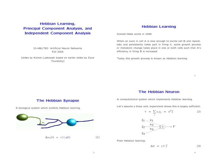
15-486/782: Artificial Neural Networks Fall 2006 (slides by Kornel Laskowski based on earlier slides by Dave Touretzky)

Hebbian Learning

Donald Hebb wrote in 1949: When an axon in cell A is near enough to excite cell B and repeat- edly and persistently takes part in firing it, some growth process

r metabolic change takes place in one or both cells such that A’s

efficiency in firing B is increased. Today this growth process is known as Hebbian learning.

2

The Hebbian Synapse

A biological system which exhibits Hebbian learning. ∆w1(t) ∝ x(t) y(t) (1)

3

The Hebbian Neuron

A computational system which implements Hebbian learning. Let’s assume a linear unit; experiment shows this is largely sufficient: V =

j

wjξj = ¯ wT ¯ ξ (2)

ξ1 ξ2 ξ3 V

w1

w2 w3

Plain Hebbian learning: ∆ ¯ w = η V ¯ ξ (3)

4

SLIDE 2

Hebbian Learning, Non-zero-mean Data

Recall that ∆ ¯ w = η V ¯ ξ and that V = ¯ wT ¯ ξ. But note that if the initial ¯ w points away from the cluster, the dot product with ¯ ξ will be negative, and ¯ w will ultimately point in exactly the opposite direction. Interpretation awkward ...

5

Plain Hebbian Learning, Zero-mean Data

Recall that ∆ ¯ w = η V ¯ ξ and that V = ¯ wT ¯ ξ. In this case, the weight vector will ultimately align itself with the direction of greatest variance in the data.

6

The Direction of Greatest Variance

If the data has zero mean, Hebbian learning will adjust the weight vector ¯ w so as to maximize the variance in the output V . When projected onto this direction, the data {¯ ξ } will exhibit variance greater than in any other direction. This direction is also known as the largest principal component of the data.

7

Locality of Plain Hebbian Learning

Looking at one synapse at a time (from input unit j) ∆wj = η V ξj (4) This is a local update rule. The Hebbian synapse, characterized by a weight wj, is modified as a function of the activity of only the two units it connects. By contrast, backprop is non-local. The update rule involves the backpropagation of a distant error signal, computed (potentially many) layers above it. This makes Hebbian learning a likely candidate for biological systems.

8

SLIDE 3

Hebbian vs Competitive Learning

Plain Competitive Learning Plain Hebbian Learning Similarities Unsupervised training methods (no teacher, no error signal). Frequently used with online learning. Strong connection to biological systems. Linear units: V = ¯ wT ¯ ξ Differences Exactly one output must be No constraint imposed by active. neighboring units. Only winner’s weights updated All weights updated at every at every epoch. epoch. ∆ ¯ w = η ¯ ξ ∆ ¯ w = η V ¯ ξ

9

A Consequence of ∆ ¯ w = η V ¯ ξ

Let’s look at the update rule Eq 3 given our expression for V in Eq 2: ∆ ¯ w = η V ¯ ξ = η

¯

wT ¯ ξ

¯

ξ (inner product) ≡ η

¯

ξ ¯ ξT ¯ w (outer product) (5) Given a current value of the weight vector ¯ w, the weight update ∆ ¯ w will be a function of the outer product of the input pattern with itself. Note that learning is incremental; that is, a weight update is per- formed each time the neuron is exposed to a training pattern ¯ ξ. We can compute an expectation for ∆ ¯ w if we take into account the distribution over patterns, P(¯ ξ ).

10

An Aside:

¯

wT ¯ ξ

¯

ξ =

¯

ξ ¯ ξT

¯

w

¯

wT ¯ ξ ¯ ξ = (w1ξ1 + w2ξ2 + · · · + wNξN)     ξ1 ξ2 . . . ξN     =     w1ξ2

1

+ w2ξ1ξ2 + · · · + wNξ1ξN w1ξ2ξ1 + w2ξ2

2

+ · · · + wNξ2ξN . . . w1ξNξ1 + w2ξNξ2 + · · · + wNξ2

N

    =     ξ2

1

ξ1ξ2 · · · ξ1ξN ξ2ξ1 ξ2

2

· · · ξ2ξN . . . . . . ... . . . ξNξ1 ξNξ2 · · · ξ2

N

        w1 w2 . . . wN     = ¯ ξ¯ ξT ¯ w

Or just

¯

wT ¯ ξ

¯

ξ = ¯ ξ

¯

wT ¯ ξ

= ¯

ξ

¯

ξT ¯ w

= ¯

ξ¯ ξT ¯ w =

¯

ξ¯ ξT ¯ w.

11

The Correlation Matrix

Taking the expectation of Eq 5 under the input distribution P(¯ ξ): ∆ ¯ w = η

¯

ξ ¯ ξT ¯ w ≡ η C ¯ w (6) where we have defined the correlation matrix as C ≡

¯

ξ ¯ ξT (7) =

     

ξ2

i

ξ1ξ2 · · · ξ1ξN ξ2ξ1 ξ2

2 · · · ξ2ξN . . . . . . ... . . . ξNξ1 ξNξ2 · · · ξ2

N      

and N is the number of inputs to our Hebbian neuron.

12

SLIDE 4

More on the Correlation Matrix

Similar to the covariance matrix Σ =

¯

ξ − ¯ µ ¯ ξ − ¯ µ

T

(8) C is the second moment of the input distribution about the origin (Σ is the second moment of the input distribution about the mean) If ¯ µ = ¯ 0, then C = Σ. Like Σ, C is symmetric. Symmetry implies that all eigenvalues are real and all eigenvectors are orthogonal. Additionally, because C is an outer product, it’s positive-definite. This means that all eigenvalues are not just real, they’re also all non-negative.

13

The Stability of Hebbian Learning

Recalling Eq 6, ∆ ¯ w = η C ¯ w From a mathematical perspective, this is a discretized version of a linear system of coupled first-order differential equations, d ¯ w dt = C ¯ w (9) whose natural solutions are ¯ w(t) = eλt ¯ u (10) where λ is a scalar and ¯ u is a vector independent of time. If we wanted to solve this system of equations, we’d still need to solve for both λ and ¯ u. There turn out to be multiple pairs {λ, ¯ u}; then ¯ w(t) is a linear combination of terms like the one in Eq 10. Note that if any λi > 0, ¯ w(t) blows up.

14

Hebbian Learning Blows Up

To see that Eq 10 represents solutions to Eq 9, C ¯ w = d ¯ w dt C

eλt ¯

u

=

d dt

eλt ¯

u

=

λ eλt ¯ u ⇒ C ¯ u = λ ¯ u (11) So the λi’s are the eigenvalues of the correlation matrix C!

1. C is an outer product ⇒ all λ ≥ 0.
2. From Eq 10, if any λ > 0 then ¯

w → ∞.

3. The λi’s cannot all be zero (true only for the zero matrix).

So plain Hebbian learning blows up.

15

Plain Hebbian Learning: Conclusions

We’ve shown that for zero-mean data, the weight vector aligns itself with the direction of maximum variance as training continues. This direction corresponds to the eigenvector of the correlation ma- trix C with the largest corresponging eigenvalue. If we decompose the current ¯ w in terms of the eigenvectors of C, ¯ w =

i αi ¯

ui, then the expected weight update rule ∆ ¯ w = η C ¯ w = η C

i

αi ¯ ui = η

i

αi λi ¯ ui (12) will move the weight vector ¯ w towards eigenvector ¯ ui by a factor proportional to λi. Over many updates, the eigenvector with the largest λi will drown out the contributions from the others. But because of this mechanism, the magnitude of ¯ w blows up.

16

SLIDE 5

Stabilizing Hebbian Learning

How to keep ¯ w from blowing up? We could renormalize ¯ w: ¯ w(τ+1)

∗

= ¯ w(τ) + ∆ ¯ w(τ) (13) ¯ w(τ+1) = ¯ w(τ+1)

∗

¯ w(τ+1)

∗

(14)

This ensures that ¯ w always has unit length. But it obliges us to give up our claim that learning is local — every synapse (wi) must know what every other synapse of the unit is doing.

17

Oja’s Rule

An alternative, suggested by Oja, is to add weight decay. The weight decay term is proportional to V 2 (recall V = ¯ wT ¯ ξ is the (output) activation of our Hebbian neuron). ∆ ¯ w = η V

¯

ξ − V ¯ w

(15)

¯ w approaches unit length, without any additional explicit effort. But it retains the property that it points in the direction of maximum variance in the data (the largest principal component).

18

Sejnowski’s Hebbian Covariance Rule

∆ ¯ w = η (V − V )

¯

ξ − ¯ ξ

(16)

Then under the input distribution P(¯ ξ), ∆ ¯ w = η

(V − V )
¯

ξ − ¯ ξ

=

η V ¯ ξ − V ¯ ξ − ¯ ξV + V ¯ ξ = η

V ¯

ξ − V ¯ ξ − V ¯ ξ + V ¯ ξ

=

η

V ¯

ξ − V ¯ ξ

=

η

¯

wT ¯ ξ

¯

ξ −

¯

wT ¯ ξ

¯

ξ

=

η

¯

ξ¯ ξT − ¯ ξ¯ ξT

¯

w (17) Subtracting the mean allows ∆ ¯ w to be negative, reducing the weight vector.

19

Principal Component Analysis (PCA)

A tool from statistics for data analysis. Can reveal structure in high-N-dimensional data that is not otherwise

bvious.

Like Hebbian learning, it discovers the direction of maximum vari- ance in the data. But then in the (N − 1)-dimensional subspace perpendicular to that direction, it discovers the direction of maxi- mum remaining variance, and so on for all N. The result is an ordered sequence of principal components. These are equivalently the eigenvectors of the correlation matrix C for zero- mean data, ordered by magnitude of eigenvalue in descending order. They are mutually orthogonal.

20

SLIDE 6

PCA: Batch Algorithm

Because of this, eigenvalue decomposition is an effective means of performing principal component analysis, if we can afford to retain all the data and do the computation offline. This is typically the case with PCA. [nData,nDim] = size(xi); xi0 = xi - ones(nData,1) * mean(xi,1); C = cov(xi0); [u,lambda] = eig(C);

21

PCA Decorrelates Data

In producing the N principal components (which are orthogonal), PCA provides an alternate, complete, orthonormal basis of N-space. ¯ ξ =

N

i=1

ξi ¯ ei =

N

i=1

ζi ¯ ui (18) ξ1 ¯ e1 + ξ2 ¯ e2 = ζ1 ¯ u1 + ζ2 ¯ u2 (19) In this basis, the data are uncorrelated.

¯ u2 ¯ ξ ζ1 ξ2 ¯ e2 ¯ ξ ξ1 ¯ e1 ζ2 ¯ u1

22

The Karhunen-Lo` eve Transform (KLT)

How do we get the ζi in Eq 18? Recall that the ¯ ui’s are orthogonal: ¯ uT

j ¯

ξ = ¯ uT

j N

i=1

ζi ¯ ui =

N

i=1

ζi ¯ uT

j ¯

ui = ζj (20) Let’s organize the ¯ ui’s as columns of a square matrix U. Then to transform all the elements of ¯ ξ at once: ¯ ζ =

    

ζ1 ζ2 . . . ζN

    

=

     

· · · ¯ uT

1 · · · · · · ¯ uT

2 · · · . . . · · · ¯ uT

N

· · ·

     

UT

    

ξ1 ξ2 . . . ξN

    

¯

ξ

(21)

23

PCA: Geometric Interpretation

The Karhunen-Lo` eve transform operates on zero-mean data; it is a function of the covariance matrix Σ only. The covariance matrix is a second-order statistic. This makes PCA a second-order method; it ignores higher-order statistics of the data. We start with the original covariance matrix in the original orthonor- mal basis. PCA applies a set of rotations to the original orthonormal basis, resulting in another orthonormal basis, such that the off-diagonal entries of the covariance matrix become zero and the diagonal entries

f the covariance matrix take on the maximum values possible.

24

SLIDE 7

Data Whitening/Sphering

The Karhunen-Lo` eve Transform ¯ ζ = UT ¯ ξ decorrelates data. This means that covariance matrix of {¯ ζ} is diagonal. We can additionally ensure the transformed data has unity covari- ance by scaling each dimension of ¯ ζ (the eigenvalues of a diagonal Σ are the variances) by the inverse of its standard deviation: ¯ ψ =

        1 √λ1

· · ·

1 √λ2

· · · . . . . . . ... . . . · · ·

1 √

λN        

√

Λ−1

UT ¯ ξ (22) Used extensively everywhere. In particular, used as a preprocessing step when training backprop networks.

25

Data Compression with PCA

If we wanted to transmit our original zero-mean dataset {¯ ξ}, we could send the zero-mean, diagonal-covariance dataset {¯ ζ} if the receiver knew the KL transform UT we used to decorrelate it. Suppose that several, say P, of the eigenvalues were very small, ie. that the contribution of the corresponding eigenvectors was (almost) statistically insignificant. Then we wouldn’t need to send the coefficients ζN−P+1 through ζN

f every datapoint for (almost) perfect reconstruction of the original

datapoint ¯ ξ. This results in a compression factor of N−P

N

(plus the overhead of communicating the N × N transform if necessary).

26

PCA with Neural Networks

We’ve seen that Hebbian learning, with appropriate provisions for preventing blow up, extracts the largest principal component. Let’s take a look at two different neural network architectures ca- pable of extracting more of them.

1. Cascading multiple Hebbian neurons.
2. Autoencoder networks (we’ve already seen these before).

27

The Hebbian Neuron, Revisited

An alternate diagram of a Hebbian neuron:

ξ1 Σ V w1 w2 w3 ξ3 ξ2

28

SLIDE 8

Extracting Multiple Principal Components

Algorithm:

1. Subtract the contribution of the first principal component.
2. Drive the difference into another Hebbian neuron.
3. This extracts the next principal component.
4. Subtract its contribution. Goto step 2.

With N Hebbian neurons, we’ll get all N principal components. Embodied in Sanger’s rule: ∆wij = η Vi

 ξj − i

k=1

Vkwkj

 

(23) This is a generalization of Oja’s rule.

29

Sanger’s Rule in Action

ξ1 ξ3 ξ2 − − − − − − − − − w11 w11 w12 w13 w13 w12 w21 w22 w23 w33 w32 w31 w21 w22 w23 w33 w32 w31

1 2 3

V3 V2 V1

30

pcademo

In matlab/pca: pcademo. Set the flag zeromean = 1 (or, incorrectly, leave zeromean to be zero for non-zero-mean data).

!! !"#$ " "#$ ! !! !"#% !"#& !"#' !"#( " "#( "#' "#& "#% ! )*+,-./01*23!24!#"""1*23(24"#5)%1*6789+4:)#$:*;+8#

31

Autoencoder Networks

We’ve already seen another neural network implementation of PCA, which we trained with backprop. It consisted of exclusively linear units.

L units M units L units

The network tries to reproduce the input in the output, inducing an short encoding in the hidden layer. This encoding retains the maxi- mum amount of information about the input in a smaller dimensional space such that the input can be reconstructed.

32

SLIDE 9

Autoencoder Networks Do PCA

It turns out that the M hidden units extract the first M principal components. Autoencoder networks can be used for dimensionality reduction, compression, etc. Because all units are linear, there is a single global minimum. Baldi (1989) has shown that there are also multiple saddle points.

33

Cottrell (1988): Image Compression

Applied the autoencoder PCA algorithm to the compression of an image. Training data consisted of 8 × 8 randomly selected patches from anywhere in the

image. Tested on entire image applying it

consecutively to all 8 × 8 non-overlapping patches. Used logistic non-linearity in the units; but claim that although the hidden units do not compute the principal components, the space they do compute is spanned by the 16 principal components.

34

Cottrell (1988): Results

The original is on the left. The right figure is a reproduction using 8 hidden units and 32 quantization levels in the hidden units. With 16 hidden units and no quantization, it is hard to tell the difference.

35

Linsker (1988): Self-Adaptive Feature Detection in Visual Cortex

Constructed a multi-layered ar- chitecture with Hebbian neurons to simulate early processing stages in the visual system. Each cell excited by an overly- ing neighborhood of cells in the previous layer.

Layer A Layer B Layer C Layer D

ENVIRONMENTAL INPUT (IF ANY) 36

SLIDE 10

Linsker (1988): Modified Hebb Rule

All cells linear, computing: V = a1 +

j

wj ξj (24) Update rule: ∆wi = a2V ξi + a3ξi + a4V + a5 (25) Cells in each layer trained to maturity before training next layer. Layer A exposed only to white noise, to understand how feature- analyzing cells could emerge even before birth in mammals.

37

Linsker (1988): Findings

Found that cells in Layer B, once matured, compute the local aver- age of the activity in the overlying region of Layer A. Due to neighborhood overlap, if one cell’s activity in Layer B happens to be high, its neighbors’ activities are also high. In Layer C, center-surround type cells emerge — responding maxi- mally to a bright spot in layer B surrounded by a dark region, and vice versa. In Layer D, orientation-selective cells emerge — responding maxi- mally to a bright edge against a dark background, and vice versa.

38

Linsker (1988): Conclusions

Receptive field map of a computed orientation-selective cell:

!!#$ !! !"#$ " "#$ ! !#$ !!#$ !! !"#$ " "#$ ! !#$

This layered construction of feature detectors is collectively due to each cell’s individual efforts to maximize the variance of its output. Each cell’s output optimally preserves the information contained in its set of input activities.

39

A Limitation of the Principle of Variance Maximization

One possibility: when the variance due to noise is high. If used for dimensionality reduction, may “accidentally” eliminate useful com- ponents and keep uninformative ones.

¯ u2 ¯ u1

40

SLIDE 11

A More Serious Limitation

Recall that PCA looks at the covariance matrix only. What if the data is not well described by the covariance matrix? The only distribution which is uniquely specified by its covariance (with the subtracted mean) is the Gaussian distribution. Distribu- tions which deviate from the Gaussian are poorly described by their covariances.

41

Faithful vs Meaningful Representations

Even with non-Gaussian data, variance maximization leads to the most faithful representation in a reconstruction error sense (recall that we trained our autoencoder network using a mean-square error in an input reconstruction layer). The mean-square error measure implicitly assumes Gaussianity, since it penalizes datapoints close to the mean less that those that are far away. But it does not in general lead to the most meaningful representa- tion. We need to perform gradient descent in some function other than the reconstruction error.

42

A Criterion Stronger than Decorrelation

The way to circumvent these problems is to look for components which are statistically independent, rather than just uncorrelated. For statistical independence, we require that p(ξ1, ξ2, · · · , ξN) =

N

i=1

p(ξi) (26) For uncorrelatedness, all we required was that ξiξj − ξi ξj = 0 , i = j (27) Independence is a stronger requirement; under independence, g1(ξi)g2(ξj) − g1(ξi) g2(ξj) = 0 , i = j (28) for any functions g1 and g2.

43

Independent Component Analysis (ICA)

Like Principal Component Analysis, except that we’re looking for a transformation subject to the stronger requirement of independence, rather than uncorrelatedness. In general, no analytic solution (like eigenvalue decomposition for PCA) exists, so ICA is implemented using neural network models. To do this, we need an architecture and an objective function to descend/climb in. Leads to N independent (or as independent as possible) components in N-dimensional space; they need not be orthogonal. When are independent components identical to uncorrelated (prin- cipal) components? When the generative distribution is uniquely determined by its first and second moments. This is true of only the Gaussian distribution.

44

SLIDE 12

Neural Network for ICA

Single layer network: Patterns {¯ ξ} are fed into the input layer. Inputs multiplied by weights in matrix W. Output logistic (vector notation here): ¯ y = 1 1 + eWT ¯

ξ

(29)

45

Objective Function for ICA

Want to ensure that the outputs yi are maximally independent. This is identical to requiring that the mutual information be small. Or alternately that the joint entropy be large.

H(p) = entropy of distribution p of first neuron’s output H(p|q) = conditional entropy I(p; q) = H(p) − H(q|p) = H(q) − H(p|q) = mutual information

Gradient ascent in this objective function is called infomax (we’re trying to maximize the enclosed area representing information quan- tities).

46

Blind Source Separation (BSS)

The most famous application of ICA. Have K sources {sk[t]}, and K signals {xk[t]}. Both {sk[t]} and {xk[t]} are time series (t is a discrete time index). Each signal is a linear mixture of the sources xk[t] = Ask[t] + nk[t] (30) where nk[t] is the noise contribution in the kth signal xk[t], and A is a mixture matrix. The problem: given xk[n], determine A and sk[n].

47

The Cocktail Party

Want to separate individual voices from a cocktail party. Here’s a 2-speaker equivalent:

)#$ ' '#$ $ $#$ & &#$ 5 <*!"

'

!! " ! =><?@A+*! )#$ ' '#$ $ $#$ & &#$ 5 <*!"

'

!! " ! =><?@A+*( )#$ ' '#$ $ $#$ & &#$ 5 <*!"

'

!! " ! 0-@A.+*B )#$ ' '#$ $ $#$ & &#$ 5 <*!"

'

!! " ! 0-@A.+*C

48

SLIDE 13

ica1,ica2,ica3

In matlab/pca. Also go to http://web.media.mit.edu/~paris/ica.html. This page has links to most of the people around the world working on ICA and BSS.

49