
SLIDE 1
ST 370 Probability and Statistics for Engineers
Hand Calculations
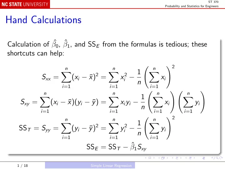
Calculation of ˆ β0, ˆ β1, and SSE from the formulas is tedious; these shortcuts can help: Sxx =
n
- i=1
(xi − ¯ x)2 =
n
- i=1
x2
i − 1
n
- n
- i=1
xi 2 Sxy =
n
- i=1
(xi − ¯ x)(yi − ¯ y) =
n
- i=1
xiyi − 1 n
- n
- i=1
xi
n
- i=1
yi
- SST = Syy =
n
- i=1
(yi − ¯ y)2 =
n
- i=1
y 2
i − 1
n
- n
- i=1
yi 2 SSE = SST − ˆ β1Sxy
1 / 18 Simple Linear Regression