gApprox: Mining Frequent Approximate Patterns from a Massive Network - - PDF document

gApprox: Mining Frequent Approximate Patterns from a Massive Network

Chen Chen† Xifeng Yan‡ Feida Zhu† Jiawei Han†

†University of Illinois at Urbana-Champaign

‡IBM T. J. Watson Research Center

{cchen37, feidazhu, hanj}@cs.uiuc.edu xifengyan@us.ibm.com

Abstract

Recently, there arise a large number of graphs with mas- sive sizes and complex structures in many new applications, such as biological networks, social networks, and the Web, demanding powerful data mining methods. Due to inherent noise or data diversity, it is crucial to address the issue of approximation, if one wants to mine patterns that are po- tentially interesting with tolerable variations. In this paper, we investigate the problem of mining fre- quent approximate patterns from a massive network and propose a method called gApprox. gApprox not only finds approximate network patterns, which is the key for many knowledge discovery applications on structural data, but also enriches the library of graph mining methodologies by introducing several novel techniques such as: (1) a com- plete and redundancy-free strategy to explore the new pat- tern space faced by gApprox; and (2) transform “frequent in an approximate sense” into an anti-monotonic constraint so that it can be pushed deep into the mining process. Sys- tematic empirical studies on both real and synthetic data sets show that frequent approximate patterns mined from the worm protein-protein interaction network are biologi- cally interesting and gApprox is both effective and efficient.

1 Introduction

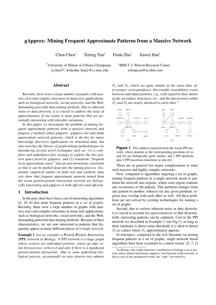
In the past, there have been a set of interesting algorithms [4, 10, 6] that mine frequent patterns in a set of graphs. Recently, there arise a large number of graphs with mas- sive sizes and complex structures in many new applications, such as biological networks, social networks, and the Web, demanding powerful data mining methods. Because of their characteristics, we are now interested in patterns that fre- quently appear at many different places of a single network. Example 1 Let us consider a Protein-Protein Interaction (PPI) network in Biology. A PPI network is a huge graph whose vertices are individual proteins, where an edge ex- ists between two vertices if and only if there is a significant protein-protein interaction. Due to some underlying bio- logical process, occasionally we may observe two subnets Pa and Pb, which are quite similar in the sense that, af- ter proper correspondence, discernable resemblance exists between individual proteins, e.g., with regard to their amino acids, secondary structures, etc., and the interactions within Pa and Pb are nearly identical to each other 1.

pqn-57 lys-1 abu-8 unc-97 F46F11.7 pqn-54 M02G9.1 abu-1 lys-2 M195.2 Y65B4A.7 F30H5.3 pqn-5

(a) (b)

ubc-18 pqn-71 ubc-1 abu-11 F35A5.4

Figure 1. Two subnets extracted from the worm PPI net-

work, where proteins at the corresponding positions of (a) and (b) are biologically quite similar, and 2 PPI deletions plus 3 PPI insertions transform (a) into (b).

There are in general two major complications to mine such massive and highly complex networks: First, compared to algorithms targeting a set of graphs, mining frequent patterns in a single network needs to par- tition the network into regions, where each region contains

• ne occurrence of the pattern. This partition changes from
• ne pattern to another; whereas for any given partition, re-

gions may overlap with each other as well. All these prob- lems are not solved by existing technologies for mining a set of graphs. Second, due to various inherent noise or data diversity, it is crucial to account for approximations so that all poten- tially interesting patterns can be captured. Cast to the PPI network we described in Example 1 (see Fig.1), as long as their similarity is above some threshold, it is ideal to detect Pb as a place where Pa approximately appears. In retrospect, compared to the rich literature on mining frequent patterns in a set of graphs, single network based algorithms have been examined to a minor extent. [5, 7, 1]

1In Biology, this might represent a mechanism to backup a set of pro-

teins whose mutual interactions support a vital function of the network, so that in case of any unexpected events, the “copy” can switch in.

took an initial step toward this direction; however, they only considered the first issue and did not pay enough attention to the second, i.e., none of them mined approximate patterns. As will be manifested later, the above two issues are actu- ally intertwined when approximation comes into play; and thus, our major challenge is to lay out a new mining para- digm that does consider approximate matching in its search space. To summarize, we made the following contributions:

• 1. We investigate the problem of mining frequent ap-

proximate patterns from a massive network: We give an ap- proximation measure and show its impact on mining, i.e., how a pattern’s support should be counted based on its ap- proximate occurrences in the network.

• 2. We propose a graph mining method called gApprox to

tackle this problem: We design a novel strategy that is both complete and redundancy-free to explore the new pattern space faced by gApprox, and transform “frequent in an ap- proximate sense” into an anti-monotonic constraint so that it can be pushed deep into the mining process.

• 3. We present systematic empirical studies on both real

and synthetic data sets: The results show that frequent ap- proximate patterns mined from the worm protein-protein in- teraction network are biologically interesting and gApprox is both effective and efficient.

• 4. The techniques we developed for gApprox are gen-

eral, which can be applied to networks from other domains, e.g., social networks. The rest of this paper is organized as follows. Section 2 presents the general model of mining frequent approximate patterns from a massive network. The mining algorithm is developed in Section 3. We report empirical studies, and give related work and discussions in Sections 4 and 5, re-

• spectively. Section 6 concludes the paper.

2 Problem Formulation

Definition 1 (Network) A network G is an edge-weighted graph, i.e., G is a 3-tuple (VG, EG, wG), where wG : EG → R+ is a weighting function mapping each edge euv = (u, v) ∈ EG to a real number wG[u, v] > 0. This setting is well-defined for many real applications, where vertices represent different entities, edges denote mu- tual relationship between entities, and weights indicate the tightness of such relationship (the tighter the relationship, the closer the two entities, and thus the smaller the weight). Definition 2 (Pattern) A pattern P is a connected and in- duced subgraph of the network G, which can be represented by a connected vertex set VP ⊆ VG.

2.1 Approximate Pattern Occurrences

The scenario we are interested in is: P, as a fragment extracted from a particular region of G, may also appear in some other regions approximately. This is associated with an injective function m : Vp → VG mapping each vertex v ∈ VP to m(v) ∈ VG. Now, to quantify the degree of approximation m incurs, we want to take into account: (1) approximation on vertices, and (2) approximation on edges. Vertex Penalties: For a vertex v ∈ VP , a list of match- able vertices matchable(v) ⊆ VG is provided. Let dis sim[v, m(v)] =

• < ∞

if m(v) ∈ matchable(v) ∞

• therwise

(0) i.e., approximations can only happen within the matchable

• list. Usually, this is a reasonable assumption in real appli-
• cations. For example, in a PPI network, though we do not

want to require that two vertices are only matchable if they represent the same protein, it is also aimless to match two proteins that are very dissimilar or even irrelevant to each

• ther. Finally, we can obtain the matchable lists by assum-

ing a similarity cut-off δ among all pairs of vertices. Edge Penalties: For a relationship (vi, vj) of P and its image (m(vi), m(vj)) under mapping m, an intuitive way to define a measure penalizing approximation is to compare the relationship tightness associated with each of them. One way of quantifying the tightness here is to plug in a short- est path based distance, which in essence treats the short- est path u v as a pseudo edge between u and v, with its weight equalling the total weight summed over u v. Now, having a (pseudo) weighted edge between each pair

• f vertices, we can simply take an absolute difference and

present the penalty function as:

• dist[vi, vj] − dist[m(vi), m(vj)]
• (1)

There could be other alternatives (e.g., max flow based) to define a distance between two vertices. Or, if the spe- cific application provides us with full tightness information among all pairs of vertices, we can directly take them as

• input. For instance, in the case of Example 1, in order to

reflect the number of PPIs that are different (i.e., present in

• ne but missing in the other) after the pattern is embedded,

we may adopt the following dist function for any two pro- teins pri and prj in the PPI network, dist[pri, prj] =

• 1

if pri and prj interact 2

• therwise

(2) since |1 − 2| = 1. In this perspective, Eq.1 and our dis- cussions below will be built on an abstract symbol of dist. Definition 3 (Degree of Approximation) Given a pattern P and a network G, an injective mapping m embeds P in some region of G by matching a vertex v ∈ VP to a vertex m(v) ∈ VG. This embedding is associated with a degree of approximation approx(P

m

− → G), which is defined as:

• v∈VP

dis sim[v, m(v)] +

• vi,vj∈VP
• dist[vi, vj] − dist[m(vi), m(vj)]
• (3)

Definition 4 (Approximate Occurrence) Given error tol- erance ∆, the vertex set {m(v)|v ∈ VP } for an embedding m is said to be an approximate occurrence of P if and only if approx(P

m

− → G) ≤ ∆.

2.2 Pattern Support with Approximation

Downward-closure is an important requirement to per- form efficient mining [9], i.e., if P is a subpattern of P ′ (VP ⊆ VP ′), then sup(P) ≥ sup(P ′) must hold. If this requirement is violated, for a task that asks for all patterns with support higher than min sup, there is no way we can stop searching for even bigger patterns at any stage during the mining process, because it is always possible for a pat- tern to qualify min sup after growing. This will make any algorithm suffer from uncontrollable explosions. Looking at Fig.2, as sup(P123) = 2 > sup(P12) = 1 if overlap- ping occurrences are counted, we have to follow a support definition in which overlaps are prohibited. Definition 5 (Pattern Support with Approximation) Two occurrences of P are said to be disjoint if and only if they do not share any vertices in common. Then, P’s pattern support with approximation is defined to be the maximal number of disjoint ones that can be chosen from the set of its approximate occurrences. Lemma 1 sup(P) ≥ sup(P ′), if P is a sub-pattern of P ′, i.e., pattern support with approximation is an anti- monotonic mining constraint. Definition 6 (Frequent Approximate Pattern Mining) Given a network G and two thresholds: (1) maximal degree

• f approximation ∆, (2) minimum support min sup, find

the pattern set P such that ∀P ∈ P, sup(P) ≥ min sup. Here, any P ∈ P is called a frequent approximate pattern.

3' 1' 3'' 2' 1 3 2 (a) (b) 1 2 P123 P12

Figure 2. Embedding patterns P123 and P12 of (a) in (b),

where 1 can match 1’, 2 can match 2’, 3 can match 3’/3”.

3 Algorithm

As a mining problem targeting all frequent approximate patterns in a network, there are two major issues we need to tackle, each of them will be discussed below.

• 1. Pattern Space Exploration: What is the problem’s

full pattern space, and how can we search through it? As we indicated in the introduction, this search space must take approximation into account.

• 2. Support Counting: For patterns in the search space,

how can we count their support and report those frequent

• nes with regard to a predetermined threshold min sup?

Based on Section 2, for each pattern, we should enumerate its approximate occurrences in the network at first, and then decide the maximal number of disjoint occurrences.

3.1 Pattern Space Exploration

As influenced by approximation, the pattern space we face here is different from that in an exact mining paradigm. Previous algorithms like [5] and [7] assume a network with vertex/edge labels, while a pattern is nothing but a labeled

• subgraph. By exact matching, in order to embed a pattern in

some region of the network, vertices/edges at corresponding positions must have identical labels. In this sense, the pat- tern space there consists of “all labeled graphs”, which can be organized on a lattice and explored by search strategies such as breadth-first search [4] and depth-first search with right-most extensions [10]. In our setting, the network is not a labeled one; to accom- modate approximations, what we have is a matchable list for each vertex indicating all vertices that are highly similar, treated as its “copies”. Keeping this in mind, it seems nec- essary for us to treat every vertex as unique, which means that each induced subgraph of the network may potentially be a different pattern, i.e., “all connected vertex sets in a given network” is our new pattern space here. In the following presentation, we are going to introduce a strategy that is both complete and redundancy-free to tra- verse the above search space. Fig.3 is taken as a running

• example. To begin with, we losslessly decompose the pat-

tern space as follows:

• 1. Find all connected vertex sets in G that contain 1.
• 2. Remove 1 from G, and find all connected vertex sets

in the new graph G that contain 2.

• 3. And so on so forth . . .

where step i explores all patterns that contain vertex i but do not contain vertices 1, 2, . . . , i−1. Now, we discuss step 1, i.e., generating all connected vertex sets starting from 1; all other steps follow the same routine. Stage 1: After the decomposition shown in Fig.3(b), start from 1 and mark 1. Stage 2: Expand from 1 to reach 2, 5, 6. Mark 2, 5, 6. There are totally seven connected vertex sets in this stage: {1,2},{1,5},{1,6},{1,2,5},{1,2,6},{1,5,6},{1,2,5,6}. In- deed, as 2, 5, 6 are all adjacent to 1, {1} union any combi- nation of 2, 5, 6 should be connected. Here, we can assume an order of 6>5>2, unrepeatedly traverse the powerset of {2,5,6} (as we do for itemsets), and finally union with {1}. The whole procedure of stage 2 is depicted in Fig.3(c). Stage 3: Taking each of the seven connected vertex sets in stage 2 as a starting point, continue expansion. In Fig.3(d), we pick {1,5,6} as an example and reach 4, 7. Mark 4, 7. Explore {1,5,6} union anything in the powerset

• f {4,7} in the same manner as we did in stage 2. Note that,

though there is an edge between 5 and 2, we prohibit the expansion to 2, because 2 has already been marked in pre- vious stages, in which case {1,5,6}{2}={1,2,5,6} is just another starting point among the seven in stage 2. More

generally, only those vertices that are both adjacent and un- marked can be absorbed during expansion.

3 4 5 1 2 6 7 3 4 5 1 2 6 7 3 4 5 2 6 7 3 4 5 6 7

…

3 4 5 1 2 6 7 3 4 5 1 2 6 7 3 4 5 1 2 6 7 3 4 5 1 2 6 7 3 4 5 1 2 6 7 3 4 5 1 2 6 7 3 4 5 1 2 6 7 3 4 5 1 2 6 7 3 4 5 1 2 6 7 3 4 5 1 2 6 7 3 4 5 1 2 6 7

(a) (b) (d) (e) (c)

Figure 3. Exploring the Pattern Space: (a) the original

graph, (b) decomposition of the problem and stage 1, (c) stage 2, (d) stage 3, (e) stage 4, where each stage is enclosed respectively within a loop. We darken marked vertices along the way, while edges are correspondingly changed from dotted to thickened as new vertices are absorbed.

Stage 4: Finally, in Fig.3(e), we pick {1,5,6,4,7} as an example from the three connected vertex sets expanded in stage 3, for which only an unmarked 3 can be absorbed. Generate {1,5,6,4,7,3} and stop expansion, because there are no more unmarked vertices now. Algorithm 1 gives pseudo-code for the above process. Theorem 1 Explore() in Algorithm 1 is both complete and redundancy-free, i.e., given a network G, (1) it only gener- ates connected vertex sets in G; (2) it can generate all con- nected vertex sets in G; (3) it does not generate the same connected vertex set more than once.

3.2 Support Counting

Now we are ready to look at support counting, in which

• ur first task is to enumerate the approximate occurrences of

any pattern encountered during Section 3.1’s pattern space

• exploration. Since Explore() follows a depth-first fashion,

which continuously absorbs new vertices and expands the current pattern P to P ′ until backtracking, we can incre- mentally obtain the occurrences of P ′ based on those of P, i.e., whenever we expand P to P ′ = P {v}, the occur- rences of P are also expanded by adding another vertex that is matchable with v. Occurrences with degree of approx- imation more than ∆ and patterns with support less than min sup are dropped immediately. A pattern P’s support is defined to be the maximal num- ber of “disjoint” ones that can be chosen from P’s approx- imate occurrences in the network. However, deciding this maximum turns out to be a very hard problem, which is re- lated to the NP-Complete maximal independent set, as some previous works have shown [5]. If it is crucial to report the “accurate frequency” of patterns, we can always calculate it by brute-force; otherwise, an upperbound, like the one developed in Algorithm 2, is enough, which will be used to stop growing patterns based on the downward-closure prop- erty. Algorithm 1 Complete and Non-redundant Exploration Function: Explore(G) Input: a network G. Output: all connected vertex sets in G. 1: for each v ∈ G do mark(v) = false; 2: pick a vertex u with smallest ID, mark(u) = true, output {u}; 3: DFS vertical(G, {u}); 4: remove u from G, and let the resulting graph be G; 5: Explore( G); Function: DFS horizontal(G, P, Vexpand) Input: a network G, a set P of connected vertices in G, a vertex set Vexpand whose powerset is to be unioned with P. Output: all connected vertex sets in G that consist of P, a proper subset of Vexpand, and some currently unmarked vertices. 1: Order the vertices in Vexpand as v1 < · · · < vk; 2: for i = 1 to k do 3: P ′ = P {vi}, output P ′; 4: V ′

expand = {vi+1, . . . , vk};

5: DFS horizontal(G, P ′, V ′

expand);

6: DFS vertical(G, P ′); Function: DFS vertical(G, P) Input: a network G, a set P of connected vertices in G. Output: all connected vertex sets in G that consist of P and some currently unmarked vertices. 1: Vexpand={v|v ∈ G, v / ∈ P, mark(v) = false, and P {v} is connected in G}; 2: for each v ∈ Vexpand do mark(v) = true; 3: DFS horizontal(G, P, Vexpand); 4: for each v ∈ Vexpand do mark(v) = false; Algorithm 2’s idea in providing an upperbound on the maximal number of disjoint ones that can be chosen from a pattern’s occurrences is explained by the following exam-

• ple. Think each occurrence as a vertex set and assume there

are 4 of them: {v1, v2}, {v1, v3}, {v1, v4}, {v2, v5}, then v1 acts like a “bottleneck” – because it is contained in 3 sets: {v1, v2}, {v1, v3}, {v1, v4}, which is the most among all 5

• vertices. Obviously, at most 1 set can be chosen from these

Algorithm 2 Providing a Support Upperbound Function: Upperbound(MP ) Input: the set of occurrences MP for a pattern P. Output: an upperbound on the maximal number of disjoint vertex sets that can be chosen from MP . 1: sup bound= 0; 2: while MP = ∅ do 3: let v be the one that appears in the greatest number

• f vertex sets in MP ;

4: sup bound=sup bound+1; 5: for each m ∈ MP do 6: if m contains v then remove m from MP ; 3 in order to ensure disjointness. Keep iterating the same procedure, we go on to consider the remaining set {v2, v5} after all sets containing v1 are removed: As we can get only 1 disjoint set here, the total number of disjoint occurrences that can be chosen is at most 1 + 1 = 2. Lemma 2 Given a pattern P, its support must be less than

• r equal to the Upperbound(MP ) provided by Algorithm 2.

Now we are ready to combine all above together and de- liver gApprox. The main skeleton of gApprox is Algorithm 1’s pattern space exploration: When examining each pat- tern encountered, i.e., on the 3rd line of DFS horizontal(), we expand the occurrences of P (i.e., MP ) to obtain those

• f P ′ (let them be MP ′), and then based on MP ′, Upper-

bound() is called to decide whether P ′ should be grown further: If not, we terminate early. In summary, gApprox is formed by simply inserting occurrence enumeration, sup- port upperbound calculation, and a conditional branch on the 3rd line of Algorithm 1’s DFS horizontal() function.

4 Experiments

We performed empirical study on both real and synthetic graph data sets. The real graph dataset is a worm PPI net- work, obtained from the DIP database (Database of Inter- acting Proteins: http://dip.doe-mbi.ucla.edu). The synthetic data generator is provided by Kuramochi et

• al. [4]. All experiments are done on a Windows machine

with 3GHz Pentium IV CPU and 1GB MEM; programs are written in C++.

4.1 Worm PPI Network

The worm PPI network contains 2,637 proteins and 4,030 PPIs. There are 12,902 pairs of matchable proteins having BLAST similarity score higher than δ = 10−7. The most “frequent” protein has 74 “copies”, while on average a protein is similar to 12902

2637 ≈ 4.9 counterparts, which sug-

gests that we must set min sup low in order to capture fre- quent patterns. We want to discover protein subnet patterns that approx- imately occur in more than min sup locations of the PPI network. As introduced in Section 2.1, Eq.1 is used to quantify the distance between any two vertices in the net-

• work. In order to focus solely on the interactions of pro-

teins, within δ, we treat the “vertex (protein) mismatch” penalty dis sim as 0. Fig.1(a) is one of the patterns discov- ered, while Fig.1(b) gives its occurrence whose degree of approximation is 5 (2 edge deletions plus 3 edge insertions). In addition to similar interconnecting topologies, the two subnetworks are composed of proteins with similar func- tions and are often from the same protein family. Pairs of functionally similar proteins are located in similar locations in the network, indicating that these two protein networks may be responsible for similar biological mechanisms. For example, proteins pqn-54 and pqn-5 have the highest de- gree in each network and are both Prion-like-(Q/N-rich)- domain-bearing proteins. The proteins adjacent to these two proteins also share similar function such as lys-1 and lys-2 which are both lysozyme proteins. Apart from pattern interestingness, we further examine the computational characteristics of gApprox. Fig.4 and Fig.5 illustrate the number of frequent approximate patterns and performance (i.e., running time) with varying minimum support (min sup) and maximal approximation (∆). It can be seen that when ∆ increases, both the running time and the number of frequent approximate patterns in- crease; while a reverse situation exists for min sup. These phenomena are well expected. Note that, in Fig.4 and Fig.5, ∆ = 4 is the maximal approximation marked on the plots; although 4 seems to be a relatively small number, it is not small indeed: From Fig.1, we can see that patterns here are in general not very “dense” networks – approximation

• n 4 PPIs means 50% error tolerance for a pattern with 8

PPIs, which is already a quite significant amount. Even though, our algorithm can still finish in about 6 minutes, which clearly demonstrates the efficiency of gApprox.

4.2 Synthetic Data

We then test gApprox on a series of synthetic data sets, showing its efficiency. The data set we take is D1T3kL200I10V60E1 [4], i.e., 1 (D) network with 3,000 (T) vertices (and 4,976 edges), which is generated by 200 (L) seed patterns of size 10 (I); the number of possible vertex and edge labels are set to 60 (V) and 1 (E), respectively. Here, two vertices are match- able (with dis sim = 0 since they are “identical”) if the same label is assigned to them. Furthermore, we randomly pick a real number from [0.5, 1] to be the weight on each edge: Since we do not want two separate vertices to have a distance close to 0, 0.5 is fixed as a lowerbound. We adopt the shortest path based distance and make a connectivity cut-off based on it. If the shortest path distance is less than 1.5, then the two vertices are considered to be connected, i.e., during pattern exploration, they are “adjacent”, and the pattern expansion from one vertex to the other is enabled.

100 1000 10000 100000 2 4 6 8 10 12

Number of Patterns Minimum Support

∆=0 ∆=1 ∆=2 ∆=3 ∆=4

Figure 4. Pattern Num-

ber w.r.t min sup and Maximal Approximation ∆, the worm PPI network

1 10 100 1000 10000 2 4 6 8 10 12

Running Time (seconds) Minimum Support

∆=0 ∆=1 ∆=2 ∆=3 ∆=4

Figure 5. Running Time

w.r.t min sup and Maxi- mal Approximation ∆, the worm PPI network

1 10 100 1000 2 4 6 8 10 12

Running Time (seconds) Minimum Support

∆=0 ∆=1 ∆=2 ∆=3 ∆=4

Figure 6. Running Time

w.r.t min sup and Maxi- mal Approximation ∆, the synthetic dataset

10 100 1000 2000 3000 4000 5000 6000

Running Time (seconds) T used in the generator

Figure 7. Running Time

w.r.t the Number of Ver- tices in the Network, the synthetic dataset

Fig.6 shows the algorithm’s performance (i.e., running time) w.r.t min sup and maximal approximation ∆; the trends are similar as those depicted in Fig.5. We then change the size of the generated network, and show how gApprox reacts (Fig.7 varies the number of vertices (T) in a network from 1000 to 5000).

5 Related Work and Discussions

Quite a few algorithms have been developed to mine fre- quent patterns over graph data [4, 10, 6]. Most of them worked on a set of graphs, which do not apply to the single graph mining scenario here. Only a few [5, 7, 1] studied the pattern mining problem in a single network. Some studies formulate the problem as a searching pro- cedure: Given a query Q, searching asks for those places where Q exactly/approximately appears in the network. Ex- act search is often referred to as graph matching, which has been actively pursued for decades [2]. Recently, a few approximate search methods have also been developed to align the query path/substructure with the subject network [3, 8], with the help of pre-built indices. However, mining is still quite different from searching in that we never know what the patterns are before discovering them. Thus, there are no pre-defined queries that can be leveraged as axles for the algorithms to search around.

6 Conclusions

In this paper, we investigate the problem of mining fre- quent approximate patterns from a massive network: We give an approximation measure and show its impact on min- ing, i.e., how a pattern’s support should be counted based on its approximate occurrences in the network. An algorithm called gApprox is presented. Empirical studies show that patterns mined from real protein-protein interaction net- works are biologically interesting and gApprox is both ef- fective and efficient. The techniques we developed for gApprox is general, which can be applied to networks from other domains as

• well. As a promising topic, it would be interesting to sys-

tematically study how gApprox can be modified to reach bigger, thus more interesting patterns even faster, with some sacrifice on the completeness of mining results.

• Acknowledgements. The work was supported in part

by the U.S. National Science Foundation NSF IIS-05- 13678/06-42771, and NSF BDI-05-15813. The authors thank Xianghong Jasmine Zhou and Michael R. Mehan for providing the cleaned PPI data and their interpretation of the patterns discovered by gApprox.

References

[1] J. Chen, W. Hsu, M.-L. Lee, and S.-K. Ng. Nemofinder: dissecting genome-wide protein-protein interactions with meso-scale network motifs. In KDD, pages 106–115, 2006. [2] D. Conte, P. Foggia, C. Sansone, and M. Vento. Thirty years of graph matching in pattern recognition. IJPRAI, 18(3):265–298, 2004. [3] M. Koyut¨ urk, A. Grama, and W. Szpankowski. Pairwise local alignment of protein interaction networks guided by models of evolution. In RECOMB, pages 48–65, 2005. [4] M. Kuramochi and G. Karypis. Frequent subgraph discov-

• ery. In ICDM, pages 313–320, 2001.

[5] M. Kuramochi and G. Karypis. Finding frequent patterns in a large sparse graph. Data Min. Knowl. Discov., 11(3):243– 271, 2005. [6] S. Nijssen and J. N. Kok. A quickstart in frequent structure mining can make a difference. In KDD, pages 647–652, 2004. [7] F. Schreiber and H. Schw¨

• bbermeyer. Frequency concepts

and pattern detection for the analysis of motifs in networks. Transactions on Computational Systems Biology, 3 (LNBI 3737):89–104, 2005. [8] Y. Tian, R. C. McEachin, C. Santos, D. J. States, and J. M. Patel. SAGA: a subgraph matching tool for biological

• graphs. Bioinformatics, pages 232–239, 2006.

[9] N. Vanetik, S. E. Shimony, and E. Gudes. Support measures for graph data. Data Min. Knowl. Discov., 13(2):243–260, 2006. [10] X. Yan and J. Han. gspan: Graph-based substructure pattern

• mining. In ICDM, pages 721–724, 2002.