Fundamental Techniques Chapter 5: Techniques 1 Outline and Reading - PowerPoint PPT Presentation
Fundamental Techniques Chapter 5: Techniques 1 Outline and Reading The Greedy Method Technique (5.1) Fractional Knapsack Problem (5.1.1) Task Scheduling (5.1.2) Divide-and-conquer paradigm (5.2) Recurrence Equations
Fundamental Techniques Chapter 5: Techniques 1
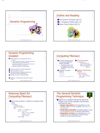
Outline and Reading The Greedy Method Technique (§5.1) Fractional Knapsack Problem (§5.1.1) Task Scheduling (§5.1.2) Divide-and-conquer paradigm (§5.2) Recurrence Equations (§5.2.1) Integer Multiplication (§5.2.2) Optional: Matrix Multiplication (§5.2.3) Dynamic Programming (§5.3) Matrix Chain-Product (§5.3.1) The General Technique (§5.3.2) 0-1 Knapsack Problem (§5.3.3) Chapter 5: Techniques 2
The Greedy Method Technique The greedy method is a general algorithm design paradigm, built on the following elements: configurations : different choices, collections, or values to find objective function : a score assigned to configurations, which we want to either maximize or minimize It works best when applied to problems with the greedy-choice property: a globally-optimal solution can always be found by a series of local improvements from a starting configuration. Chapter 5: Techniques 3
Making Change Problem: A dollar amount to reach and a collection of coin amounts to use to get there. Configuration: A dollar amount yet to return to a customer plus the coins already returned Objective function: Minimize number of coins returned. Greedy solution: Always return the largest coin you can Example 1: Coins are valued $.32, $.08, $.01 Has the greedy-choice property, since no amount over $.32 can be made with a minimum number of coins by omitting a $.32 coin (similarly for amounts over $.08, but under $.32). Example 2: Coins are valued $.30, $.20, $.05, $.01 Does not have greedy-choice property, since $.40 is best made with two $.20’s, but the greedy solution will pick three coins (which ones?) Chapter 5: Techniques 4
The Fractional Knapsack Problem Given: A set S of n items, with each item i having b i - a positive benefit w i - a positive weight Goal: Choose items with maximum total benefit but with weight at most W. If we are allowed to take fractional amounts, then this is the fractional knapsack problem . In this case, we let x i denote the amount we take of item i ∑ b ( x / w ) Objective: maximize i i i ∈ S i ∑ ≤ x W Constraint: i ∈ i S Chapter 5: Techniques 5
Example Given: A set S of n items, with each item i having b i - a positive benefit w i - a positive weight Goal: Choose items with maximum total benefit but with weight at most W. “knapsack” Solution: • 1 ml of 5 Items: • 2 ml of 3 1 2 3 4 5 • 6 ml of 4 Weight: 4 ml 8 ml 2 ml 6 ml 1 ml • 1 ml of 2 Benefit: $12 $32 $40 $30 $50 10 ml Value: 3 4 20 5 50 ($ per ml) Chapter 5: Techniques 6
The Fractional Knapsack Algorithm Greedy choice: Keep taking item with highest value (benefit to Algorithm fractionalKnapsack ( S, W ) weight ratio) Input: set S of items w/ benefit b i Since ∑ ∑ = and weight w i ; max. weight W b ( x / w ) ( b / w ) x i i i i i i Output: amount x i of each item i ∈ ∈ i S i S Run time: O(n log n). See P . 260 to maximize benefit with Knapsack satisfies Greedy-Choice weight at most W Property: for each item i in S there is an item i with higher x i ← 0 value than a chosen item j (i.e., v i ← b i / w i vi> vj) but x i < w i and x j > 0 If we {value} substitute some i with j, we get a w ← 0 {total weight} better solution while w < W How much of i: y= min{ w i -x i , x j } . Thus we can replace y of item j remove item i with highest v i with an equal amount of item I, x i ← min{ w i , W − w } which is the greedy choice w ← w + min{ w i , W − w } property. Chapter 5: Techniques 7
Task Scheduling Given: a set T of n tasks, each having: A start time, s i A finish time, f i (where s i < f i ) Goal: Perform all the tasks using a minimum number of “machines.” Note only one task per machine at atime. Machine 3 Machine 2 Machine 1 1 2 3 4 5 6 7 8 9 Chapter 5: Techniques 8
Task Scheduling Algorithm Greedy choice: consider tasks by their start time and use as few machines as possible with Algorithm taskSchedule ( T ) this order. Input: set T of tasks w/ start time s i Run time: O(n log n). Why? and finish time f i Correctness: Suppose there is a Output: non-conflicting schedule better schedule. with minimum number of machines m ← 0 We can use k-1 machines {no. of machines} while T is not empty The algorithm uses k remove task i w/ smallest s i Let i be first task scheduled if there’s a machine j for i then on machine k schedule i on machine j Machine i must conflict with else k-1 other tasks m ← m + 1 But that means there is no schedule i on machine m non-conflicting schedule using k-1 machines Chapter 5: Techniques 9
Example Given: a set T of n tasks, each having: A start time, s i A finish time, f i (where s i < f i ) [1,4], [1,3], [2,5], [3,7], [4,7], [6,9], [7,8] (ordered by start) Goal: Perform all tasks on min. number of machines Machine 3 Machine 2 Machine 1 1 2 3 4 5 6 7 8 9 Chapter 5: Techniques 10
Divide-and-Conquer 7 2 9 4 → 2 4 7 9 7 2 → 2 7 9 4 → 4 9 7 → 7 2 → 2 9 → 9 4 → 4 Chapter 5: Techniques 11
Divide-and-Conquer Divide-and conquer is a general algorithm design paradigm: Divide: divide the input data S in two or more disjoint subsets S 1 , S 2 , … Recur: solve the subproblems recursively Conquer: combine the solutions for S 1 , S 2 , …, into a solution for S The base case for the recursion are subproblems of constant size Analysis can be done using recurrence equations Chapter 5: Techniques 12
Merge-Sort Review Merge-sort on an input sequence S with n Algorithm mergeSort ( S, C ) elements consists of Input sequence S with n three steps: elements, comparator C Divide: partition S into Output sequence S sorted two sequences S 1 and S 2 according to C of about n / 2 elements if S.size () > 1 each ( S 1 , S 2 ) ← partition ( S , n /2) Recur: recursively sort S 1 mergeSort ( S 1 , C ) and S 2 mergeSort ( S 2 , C ) Conquer: merge S 1 and S ← merge ( S 1 , S 2 ) S 2 into a unique sorted sequence Chapter 5: Techniques 13
Recurrence Equation Analysis The conquer step of merge-sort consists of merging two sorted sequences, each with n / 2 elements and implemented by means of a doubly linked list, takes at most bn steps, for some constant b . Likewise, the basis case ( n < 2) will take at b most steps. Therefore, if we let T ( n ) denote the running time of merge-sort: < b if n 2 = T ( n ) + ≥ 2 T ( n / 2 ) bn if n 2 We can therefore analyze the running time of merge-sort by finding a closed form solution to the above equation. That is, a solution that has T ( n ) only on the left-hand side. Chapter 5: Techniques 14
Iterative Substitution In the iterative substitution, or “plug-and-chug,” technique, we iteratively apply the recurrence equation to itself and see if we can = + find a pattern: T ( n ) 2 T ( n / 2 ) bn = + + 2 2 ( 2 T ( n / 2 )) b ( n / 2 )) bn = + 2 2 2 T ( n / 2 ) 2 bn = + 3 3 2 T ( n / 2 ) 3 bn = + 4 4 2 T ( n / 2 ) 4 bn = ... = + i i 2 T ( n / 2 ) ibn Note that base, T(n)= b, case occurs when 2 i = n. That is, i = log n. So, = + T ( n ) bn bn log n Thus, T(n) is O(n log n). Chapter 5: Techniques 15
The Recursion Tree Draw the recursion tree for the recurrence relation and look for a pattern: < b if n 2 = T ( n ) + ≥ 2 T ( n / 2 ) bn if n 2 time depth T’s size bn 0 1 n bn n / 2 1 2 n / 2 i bn 2 i i … … … … Total time = bn + bn log n (last level plus all previous levels) Chapter 5: Techniques 16
Guess-and-Test Method In the guess-and-test method, we guess a closed form solution and then try to prove it is true by induction: < b if n 2 = T ( n ) + ≥ 2 T ( n / 2 ) bn log n if n 2 Guess: T(n) < cn log n. = + T ( n ) 2 T ( n / 2 ) bn log n = + 2 ( c ( n / 2 ) log( n / 2 )) bn log n = − + cn (log n log 2 ) bn log n = − + cn log n cn bn log n Wrong: we cannot make this last line be less than cn log n Chapter 5: Techniques 17
Guess-and-Test Method, Part 2 Recall the recurrence equation: < b if n 2 = T ( n ) + ≥ 2 T ( n / 2 ) bn log n if n 2 Guess # 2: T(n) < cn log 2 n. = + T ( n ) 2 T ( n / 2 ) bn log n = + 2 2 ( c ( n / 2 ) log ( n / 2 )) bn log n = − + 2 cn (log n log 2 ) bn log n = − + + 2 cn log n 2 cn log n cn bn log n ≤ 2 cn log n if c > b. So, T(n) is O(n log 2 n). In general, to use this method, you need to have a good guess and you need to be good at induction proofs. Chapter 5: Techniques 18
Recommend


More recommend
Explore More Topics
Stay informed with curated content and fresh updates.