
SLIDE 1
Alexandre Girouard
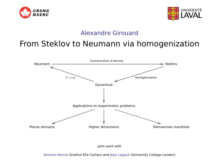
From Steklov to Neumann via homogenization
Neumann
Concentration of density
Steklov
Homogenization
- Dynamical
β→∞
- Applications to isoperimetric problems
- Planar domains
Higher dimensions Riemannian manifolds joint work with Antoine Henrot (Institut Elie Cartan) and Jean Lagacé (University College London)