
SLIDE 1
From Movement Tracks From Movement Tracks through Events to Places: - - PowerPoint PPT Presentation
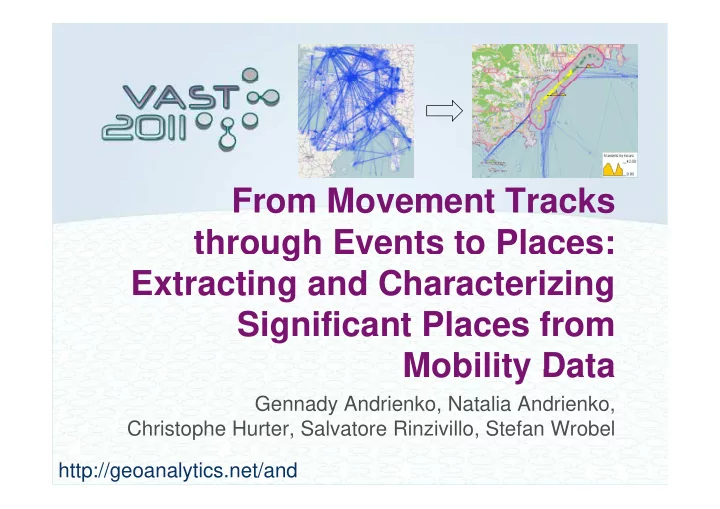
From Movement Tracks From Movement Tracks through Events to Places: g Extracting and Characterizing Si Significant Places from ifi t Pl f Mobility Data Mobility Data Gennady Andrienko, Natalia Andrienko, Christophe Hurter Salvatore
Find dense spatial clusters of events, taking into account time and attributes Find dense spatial clusters of events, taking into account time and attributes Events, trajectories places + time series of attribute values Events, trajectories places + time series of attribute values Surround clusters with spatial buffers Surround clusters with spatial buffers Trajectories flows between places Trajectories flows between places with spatial buffers with spatial buffers
place 2> + time series
The trajectories are drawn
1 2 3 4
1 2 3 4
Each trajectory is represented by a horizontal segmented bar. Th t l d di t th tt ib t l The segments are colored according to the attribute values. Information about the segment The popup window shows attributes of the whole trajectory that is pointed with the mouse cursor. Information about the segment pointed by the mouse cursor is shown on the top of the window. trajectory that is pointed with the mouse cursor. The user interactively breaks the value range into
Time
The user interactively breaks the value range into intervals (classes) and can choose the color scale. The colors are used to paint bar segments.
1 2 3 4
The user clicks on a rectangle in the legend to switch off the Only the bar segments representing respective interval or to switch it on again. Only the bar segments representing values from the currently active interval(s) are shown. The map shows only the points and segments of the trajectories where the values
y y Here we see the points and segments where the speed was not more than 10 km/h.
1 2 3 4
This button in the “data” tab allows the user to This button in the data tab allows the user to extract m-events from the trajectories according to the current segment filter. The extracted events are organized in a new dataset consisting of points and multi-points with time references and tt ib t attributes. The map shows the extracted low speed events as an independent map layer. The m-events are represented by red hollow circles. y
1 2 3 4
1 2 3 4
t t if t t t t if t t t t d
end start end start start end end start t
) 1 ( ) (
2 1 2 1 2 1 1 2 2 1
f
t
) ( ) (
2 1 2 1 2 , 1
1, 2, |1 2|, |1 2| 2 ⁄
|
∃ | ,
2,
, … ,
∗
2 2
3
1 2 3 4
The result of the density- based clustering of the events by their spatial positions, temporal positions and temporal positions, and movement directions (STD) with the distance thresholds 100 meters, 10 minutes, and 20 degrees and the minimum 20 degrees and the minimum number of neighbors 5. Gray color represents “ i ” i t th t “noise”, i.e., events that have not enough neighbors and therefore have not been put in l t clusters. We filter the noise out using the checkbox.
1 2 3 4
1 2 3 4
The space-time cube is viewed from the north.
North North
1 2 3 4
The second stage of the clustering is applied only to the objects belonging to the STD-clusters, i.e., without the “noise” without the noise .
1 2 3 4
The SD-clustering has united STD-clusters that united STD-clusters that
but overlap in space.
North
1 2 3 4
The places are painted according to the prevailing movement directions of the respective events. respective events.
Belt road north-south on the east of the city (A50)
1 2 3 4
Belt road north-south on the east of the city (A50) Extended areas of congested traffic di t d t th th directed to the south and southeast Belt road west-east on the north of the city (A4) Smaller areas of
directed to the north and northwest Very long area of congested traffic and northwest directed to the east Long area of congested movements directed to the west
1 2 3 4
1 2 3 4
1 2 3 4
The temporal diagrams show the variation of the attribute value (vertical dimension)
dimension) dimension).
1 2 3 4
Congested traffic in the afternoon in the direction
Congested traffic in the morning in the direction to the south
1 2 3 4
Northeast East
i d idd
Northeast
morning morning and midday morning morning and afternoon morning and afternoon afternoon morning afternoon
The trajectories are drawn
1 2 3 4
1 2 3 4
1 2 3 4
1 2 3 4
1 2 3 4
Cl t b Clusters by spatial positions (S) and directions (D). The noise has been hidden.
1 2 3 4
Nice
Changes of the landing direction at Nice
1 2 3 4
1 2 3 4
1 2 3 4
2 3 4
F th th t From the northeast: from 13 till 16 o’clock From the southwest: morning till midday and then starting from 17 o’clock Lines represent last 10 minutes
1 2 3 4
1 2 3 4
1 2 3 4
1 2 3 4
1 2 3 4
1 2 3 4
The arrows represent aggregate moves (flows) between areas. Th thi k i ti l The thickness is proportional to the total number of flights. The colors represent the directions.
Paris
Minor flows (less than 5 flights) have been hidden. A di l t t f th i A radial structure of the air traffic is visible (Paris periphery). Different airports in Paris may p y be used for flights to/from the same city (e.g., Bordeaux, Toulouse, Marseille, Nice)
Bordeaux Toulouse Marseille Nice
1 2 3 4
1 2 3 4
Th d t th t fl i i f l Th l d t th The rows correspond to the aggregate flows, i.e., pairs of places. The columns correspond to the time intervals used for the aggregation. The flow counts are represented by proportional lengths
connections Marseille Paris Orly (yellow) and Paris Orly Marseille (orange) are highlighted. y (y ) y ( g ) g g
1 2 3 4
One or two flights every hour between 08h and 18h except 15h Three flights every hour from 22h to 24h
Marseille Paris Orly Paris Orly Paris Orly Marseille
Three flights per hour at 01h and 02h One flight per hour in intervals 07h, 08h, from 11h to14h, 19h, 20h
y, g g , , , * appropriate similarity measures
All steps could be scaled up by database All steps could be scaled up by database processing