
SLIDE 1
Department of Chemical Engineering I.I.T. Bombay, India
Frequency Response Response of the process to signals of varying - - PowerPoint PPT Presentation
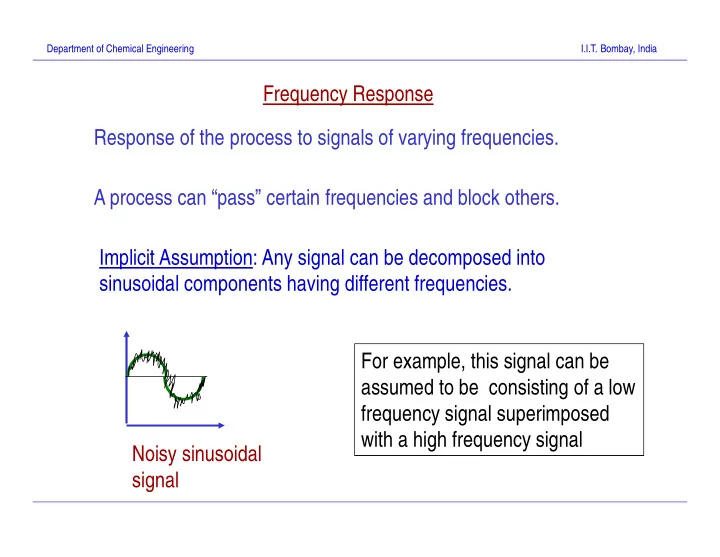
Department of Chemical Engineering I.I.T. Bombay, India Frequency Response Response of the process to signals of varying frequencies. A process can pass certain frequencies and block others. Implicit Assumption: Any signal can be
Department of Chemical Engineering I.I.T. Bombay, India
Department of Chemical Engineering I.I.T. Bombay, India
Department of Chemical Engineering I.I.T. Bombay, India
Department of Chemical Engineering I.I.T. Bombay, India
2 2
2 2
Department of Chemical Engineering I.I.T. Bombay, India
Real axis
b a
Department of Chemical Engineering I.I.T. Bombay, India
Department of Chemical Engineering I.I.T. Bombay, India
2 2 2 2 2 2
2 2 2 2
2 2 2 2 2 2
2 2
Department of Chemical Engineering I.I.T. Bombay, India
Department of Chemical Engineering I.I.T. Bombay, India
Department of Chemical Engineering I.I.T. Bombay, India
Department of Chemical Engineering I.I.T. Bombay, India
Department of Chemical Engineering I.I.T. Bombay, India
1
2 2
w K
) ( tan 1 w
) 1 log( 2 1 ) log(
2 2
w K AR
Department of Chemical Engineering I.I.T. Bombay, India
1
Department of Chemical Engineering I.I.T. Bombay, India
1 2 2
Department of Chemical Engineering I.I.T. Bombay, India
1 1 2 2 2 2
Effective Lag Effective Lead
Department of Chemical Engineering I.I.T. Bombay, India
2 2 2 2 1 2 2 2 2 2 1 2 2 1 2 1
Department of Chemical Engineering I.I.T. Bombay, India
2 2 1 2 2 2 2 2 2
Effect of damping factor
Transfer Function
2
r
Department of Chemical Engineering I.I.T. Bombay, India
Department of Chemical Engineering I.I.T. Bombay, India
jw s