Fredholm Determinants: 2 , 000 A Robust 0 Approach to 2 , 000 - - PowerPoint PPT Presentation

Fredholm Determinants: A Robust Approach to Computing Stokes Eigenvalues

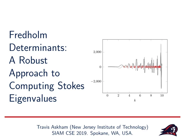
2 4 6 8 10 −2,000 2,000 k

Travis Askham (New Jersey Institute of Technology) SIAM CSE 2019. Spokane, WA, USA.

Joint work with Manas Rachh (Flatiron Institute) Barnett, Greengard

Stokes Eigenvalues

−∆u + ∇p = k2u in Ω ∇ · u = 0 in Ω u = 0 on ∂Ω

Stokes Eigenvalues

−∆u + ∇p = k2u in Ω ∇ · u = 0 in Ω u = 0 on ∂Ω Stability of steady flows

Stokes Eigenvalues

−∆u + ∇p = k2u in Ω ∇ · u = 0 in Ω u = 0 on ∂Ω Stability of steady flows Decay of turbulent flows

Stokes Eigenvalues

−∆u + ∇p = k2u in Ω ∇ · u = 0 in Ω u = 0 on ∂Ω Stability of steady flows Decay of turbulent flows History of studying the spectrum

Related Problem: Buckling Eigenvalues

Related Problem: Buckling Eigenvalues

Stream function u = ∇⊥Ψ

Related Problem: Buckling Eigenvalues

Stream function u = ∇⊥Ψ Stokes eigenvalue problem becomes −∆2Ψ = k2∆Ψ in Ω ∇Ψ = 0 on ∂Ω

Related Problem: Buckling Eigenvalues

Stream function u = ∇⊥Ψ Stokes eigenvalue problem becomes −∆2Ψ = k2∆Ψ in Ω ∇Ψ = 0 on ∂Ω The buckling problem −∆2Ψ = k2∆Ψ in Ω Ψ = ∂νΨ = 0 on ∂Ω

Buckling Eigenvalues

[fetraining.net]

Buckling Eigenvalues

First eigenvalue describes buckling load of an idealized elastic plate under compression

[fetraining.net]

Buckling Eigenvalues

First eigenvalue describes buckling load of an idealized elastic plate under compression Equivalent to Stokes eigenvalues

• n simply-connected domains

[fetraining.net]

Buckling Eigenvalues

First eigenvalue describes buckling load of an idealized elastic plate under compression Equivalent to Stokes eigenvalues

• n simply-connected domains

Of pure mathematical interest:

[fetraining.net]

Buckling Eigenvalues

First eigenvalue describes buckling load of an idealized elastic plate under compression Equivalent to Stokes eigenvalues

• n simply-connected domains

Of pure mathematical interest:

Relation to Laplace (membrane) eigenvalues/ eigenfunctions

[Antunes 2011]

Buckling Eigenvalues

First eigenvalue describes buckling load of an idealized elastic plate under compression Equivalent to Stokes eigenvalues

• n simply-connected domains

Of pure mathematical interest:

Relation to Laplace (membrane) eigenvalues/ eigenfunctions Intricate structure of eigenfunctions on domains with corners

[Antunes 2011] [Leriche and Labrosse 2004]

Approximating Drum, Stokes, and Buckling Eigenvalues

Approximating Drum, Stokes, and Buckling Eigenvalues

Pen and paper: Rayleigh, A. Weinstein, P´

• lya, Szeg¨
• , Payne,

Rellich

Approximating Drum, Stokes, and Buckling Eigenvalues

Pen and paper: Rayleigh, A. Weinstein, P´

• lya, Szeg¨
• , Payne,

Rellich Finite elements and spectral methods dominate: Babuska, Osborn, Ciarlet, Q. Lin, Dur´ an, J. Shen, Boyd

Approximating Drum, Stokes, and Buckling Eigenvalues

Pen and paper: Rayleigh, A. Weinstein, P´

• lya, Szeg¨
• , Payne,

Rellich Finite elements and spectral methods dominate: Babuska, Osborn, Ciarlet, Q. Lin, Dur´ an, J. Shen, Boyd Method of fundamental solutions and other compact operator approaches: Kupradze and Aleksidze 1964; Kitahara 1985; Antunes 2011

Approximating Drum, Stokes, and Buckling Eigenvalues

Pen and paper: Rayleigh, A. Weinstein, P´

• lya, Szeg¨
• , Payne,

Rellich Finite elements and spectral methods dominate: Babuska, Osborn, Ciarlet, Q. Lin, Dur´ an, J. Shen, Boyd Method of fundamental solutions and other compact operator approaches: Kupradze and Aleksidze 1964; Kitahara 1985; Antunes 2011 Second-kind equations: B¨ acker 2003, Bornemann 2010 (Nystr¨

• m discretization of Fredholm determinant); Zhao and

Barnett 2014 (drum); Lindsay, Quaife, and Wendelberger 2018 (mode elimination a la Farkas)

Computing Eigenvalues: 2 Approaches

−∆u = k2u in Ω u = 0 on ∂Ω

Computing Eigenvalues: 2 Approaches

−∆u = k2u in Ω u = 0 on ∂Ω

Eigenvalues of Discretization

− ∆u = k2u in Ω u = 0 on ∂Ω ↓ ANuN = k2BNuN ↓ kN =

• eig(AN, BN)

Computing Eigenvalues: 2 Approaches

−∆u = k2u in Ω u = 0 on ∂Ω

Eigenvalues of Discretization

− ∆u = k2u in Ω u = 0 on ∂Ω ↓ ANuN = k2BNuN ↓ kN =

• eig(AN, BN)

Discretization of Eigenvalue Indicator

u = −2D(k)µ ↓ dim(N(I − 2D(k))) > 0 ⇐ ⇒ k eval ↓ f(k) = det(I − 2D(k)) = 0 ↓ k = roots(fN)

Why use the Eigenvalue Indicator Approach? And Why Insist on Second-Kind Equations?

Why use the Eigenvalue Indicator Approach? And Why Insist on Second-Kind Equations?

Direct PDE discretization suffers from high frequency pollution and ill-conditioning

Why use the Eigenvalue Indicator Approach? And Why Insist on Second-Kind Equations?

Direct PDE discretization suffers from high frequency pollution and ill-conditioning First kind equations and the method of fundamental solutions don’t have good, convergent indicators of non-invertibility — the test of an eigenvalue is relative to the discretization

Why use the Eigenvalue Indicator Approach? And Why Insist on Second-Kind Equations?

Direct PDE discretization suffers from high frequency pollution and ill-conditioning First kind equations and the method of fundamental solutions don’t have good, convergent indicators of non-invertibility — the test of an eigenvalue is relative to the discretization Fast direct methods behave well for second-kind equations

Why use the Eigenvalue Indicator Approach? And Why Insist on Second-Kind Equations?

Direct PDE discretization suffers from high frequency pollution and ill-conditioning First kind equations and the method of fundamental solutions don’t have good, convergent indicators of non-invertibility — the test of an eigenvalue is relative to the discretization Fast direct methods behave well for second-kind equations Straightforward to make high order tools

Why use the Eigenvalue Indicator Approach? And Why Insist on Second-Kind Equations?

Direct PDE discretization suffers from high frequency pollution and ill-conditioning First kind equations and the method of fundamental solutions don’t have good, convergent indicators of non-invertibility — the test of an eigenvalue is relative to the discretization Fast direct methods behave well for second-kind equations Straightforward to make high order tools Down the line — for certain second kind kernels, corners can be handled robustly/efficiently a la Serkh et al. or Helsing

“drum eigenvalues” −∆u = k2u in Ω u = 0 on ∂Ω

image: bio physics wiki

Zhao and Barnett Program

“drum eigenvalues” −∆u = k2u in Ω u = 0 on ∂Ω

image: bio physics wiki

Zhao and Barnett Program

Reformulate as second-kind integral equation I − 2D(k)

“drum eigenvalues” −∆u = k2u in Ω u = 0 on ∂Ω

image: bio physics wiki

Zhao and Barnett Program

Reformulate as second-kind integral equation I − 2D(k) Nystr¨

• m discretize to high

accuracy IN − 2DN(k)

“drum eigenvalues” −∆u = k2u in Ω u = 0 on ∂Ω

image: bio physics wiki

Zhao and Barnett Program

Reformulate as second-kind integral equation I − 2D(k) Nystr¨

• m discretize to high

accuracy IN − 2DN(k) Approximate Fredholm determinant (an analytic function) fN(k) = det(IN − 2DN(k))

“drum eigenvalues” −∆u = k2u in Ω u = 0 on ∂Ω

image: bio physics wiki

Zhao and Barnett Program

Reformulate as second-kind integral equation I − 2D(k) Nystr¨

• m discretize to high

accuracy IN − 2DN(k) Approximate Fredholm determinant (an analytic function) fN(k) = det(IN − 2DN(k)) Use high-order root finding on fN(k) to obtain eigenvalues

“drum eigenvalues” −∆u = k2u in Ω u = 0 on ∂Ω

image: bio physics wiki

Zhao and Barnett Program

Reformulate as second-kind integral equation I − 2D(k) Nystr¨

• m discretize to high

accuracy IN − 2DN(k) Approximate Fredholm determinant (an analytic function) fN(k) = det(IN − 2DN(k)) Use high-order root finding on fN(k) to obtain eigenvalues On multiply-connected / exterior resonance, replace D with combined field

The ZB Program for Stokes

The ZB Program for Stokes

Develop a second kind representation for Stokes EV problem, u = K(k)µ

The ZB Program for Stokes

Develop a second kind representation for Stokes EV problem, u = K(k)µ Establish that { eigenvalues } = {k : dim(N(I − K(k))) > 0}

The ZB Program for Stokes

Develop a second kind representation for Stokes EV problem, u = K(k)µ Establish that { eigenvalues } = {k : dim(N(I − K(k))) > 0} Discretization and solution is “off-the-shelf”

Oscillatory Stokes BVPs

Oscillatory Stokes BVPs

Interior Dirichlet Problem

−∆u + ∇p = k2u in Ω ∇ · u = 0 in Ω u = f on Γ Compatibility condiiton

• Γ ν · f dS = 0.

Oscillatory Stokes BVPs

Interior Dirichlet Problem

−∆u + ∇p = k2u in Ω ∇ · u = 0 in Ω u = f on Γ Compatibility condiiton

• Γ ν · f dS = 0.

Interior Neumann Problem

−∆u + ∇p = k2u in Ω ∇ · u = 0 in Ω σ(u, p) = g on Γ

Oscillatory Stokeslets

−(∆ + k2)u + ∇p = δy(x)f in Ω ∇ · u = 0 in Ω

Oscillatory Stokeslets

−(∆ + k2)u + ∇p = δy(x)f in Ω ∇ · u = 0 in Ω GL(x, y) = −log |x − y| 2π ⇒ ∆GL = δy(x)

Oscillatory Stokeslets

−(∆ + k2)u + ∇p = δy(x)f in Ω ∇ · u = 0 in Ω GL(x, y) = −log |x − y| 2π ⇒ ∆GL = δy(x) ↓ ⇒ p = ∇GL · f

Oscillatory Stokeslets

−(∆ + k2)u + ∇p = δy(x)f in Ω ∇ · u = 0 in Ω GL(x, y) = −log |x − y| 2π ⇒ ∆GL = δy(x) ↓ ⇒ p = ∇GL · f ↓ −(∆ + k2)u = ∆GLf − ∇(∇GL · f)

Oscillatory Stokeslets

−(∆ + k2)u + ∇p = δy(x)f in Ω ∇ · u = 0 in Ω GL(x, y) = −log |x − y| 2π ⇒ ∆GL = δy(x) ↓ ⇒ p = ∇GL · f ↓ −(∆ + k2)u = ∆GLf − ∇(∇GL · f) ↓ u = ((∇ ⊗ ∇ − ∆I)GBH)f = −(∇⊥⊗∇⊥GBH)f

Oscillatory Stokeslets

−(∆ + k2)u + ∇p = δy(x)f in Ω ∇ · u = 0 in Ω GL(x, y) = −log |x − y| 2π ⇒ ∆GL = δy(x) ↓ ⇒ p = ∇GL · f ↓ −(∆ + k2)u = ∆GLf − ∇(∇GL · f) ↓ u = ((∇ ⊗ ∇ − ∆I)GBH)f = −(∇⊥⊗∇⊥GBH)f where

GBH(x, y; k) = 1 k2 1 2π log |x − y| + i 4 H1

0(k|x − y|)

• ∆(∆ + k2)GBH = δ

Stresslet

Stresslet

Let G(k)(x, y) = (∇ ⊗ ∇ − ∆I)GBH(x, y; k).

Stresslet

Let G(k)(x, y) = (∇ ⊗ ∇ − ∆I)GBH(x, y; k). u(x) = G(k)(x, y)f , p(x) = ∇GL(x, y) · f

Stresslet

Let G(k)(x, y) = (∇ ⊗ ∇ − ∆I)GBH(x, y; k). u(x) = G(k)(x, y)f , p(x) = ∇GL(x, y) · f The stress tensor is σ(x) = −p(x)I + ∇u(x) + (∇u(x))⊺ =: T(k)f

Stresslet

Let G(k)(x, y) = (∇ ⊗ ∇ − ∆I)GBH(x, y; k). u(x) = G(k)(x, y)f , p(x) = ∇GL(x, y) · f The stress tensor is σ(x) = −p(x)I + ∇u(x) + (∇u(x))⊺ =: T(k)f Stresslet Tijℓ = −∂xjGLδiℓ + ∂xℓ

• −∆GBHδij + ∂xi
• ∂xjGBH

Layer Potentials

Ω Γ = ∂Ω

ν is normal to boundary

Layer Potentials

Ω Γ = ∂Ω

ν is normal to boundary Single S(k)[µ](x) =

• Γ

G(k)(x, y)µ(y) dS(y)

Layer Potentials

Ω Γ = ∂Ω

ν is normal to boundary Single S(k)[µ](x) =

• Γ

G(k)(x, y)µ(y) dS(y) Double D(k)[µ](x) =

• Γ
• T(k)

·,·,ℓ(x, y)νℓ(y)

⊺ µ(y) dS(y)

S(k) single layer σ(k)

S

stress of single layer off boundary D(k) double layer off boundary D(k) double layer on boundary N (k) = D(k)⊺ stress of single layer on boundary

S(k) single layer σ(k)

S

stress of single layer off boundary D(k) double layer off boundary D(k) double layer on boundary N (k) = D(k)⊺ stress of single layer on boundary

Lemma (Jump conditions)

For a given density µ defined on Γ, Sµ is continuous across Γ, the exterior and interior limits of the surface traction of Dµ are equal, and for each x0 ∈ Γ, lim

h↓0 σ(k) S [µ](x0 ± hν(x0)) · ν(x0) = ∓1

2µ(x0) + N (k)[µ](x0) lim

h↓0 D(k)[µ](x0 ± hν(x0)) = ±1

2µ(x0) + D(k)[µ](x0) .

Setting u(x) = D(k)[µ](x) the Dirichlet problem becomes −1 2µ + D(k)µ = f on Γ

Setting u(x) = D(k)[µ](x) the Dirichlet problem becomes −1 2µ + D(k)µ = f on Γ

Note: dim(N(− 1

2 + D(k))) > 0 for any k

(µ, (− 1

2 + N (k))ν) = (− 1 2 + D(k))µ, ν) = 0 for all µ, i.e.

(− 1

2 + N (k))ν = 0.

Nullspace Correction

Definition

W[µ](x) = 1 |Γ|

• Γ

ν(x)(ν(y) · µ(y)) dS(y)

Nullspace Correction

Definition

W[µ](x) = 1 |Γ|

• Γ

ν(x)(ν(y) · µ(y)) dS(y) Properties W[W[µ]] = W[µ] W[1/2 ± D(k)] = 0 W[S(k)] = 0

Nullspace Correction

Definition

W[µ](x) = 1 |Γ|

• Γ

ν(x)(ν(y) · µ(y)) dS(y) Properties W[W[µ]] = W[µ] W[1/2 ± D(k)] = 0 W[S(k)] = 0 Adding W Doesn’t change equation for compatible f

Nullspace Correction

Definition

W[µ](x) = 1 |Γ|

• Γ

ν(x)(ν(y) · µ(y)) dS(y) Properties W[W[µ]] = W[µ] W[1/2 ± D(k)] = 0 W[S(k)] = 0 Adding W Doesn’t change equation for compatible f − 1 2µ + D(k)µ + Wµ = f

Nullspace Correction

Definition

W[µ](x) = 1 |Γ|

• Γ

ν(x)(ν(y) · µ(y)) dS(y) Properties W[W[µ]] = W[µ] W[1/2 ± D(k)] = 0 W[S(k)] = 0 Adding W Doesn’t change equation for compatible f − 1 2µ + D(k)µ + Wµ = f W(−1 2µ + D(k)µ + Wµ) = W[f]

Nullspace Correction

Definition

W[µ](x) = 1 |Γ|

• Γ

ν(x)(ν(y) · µ(y)) dS(y) Properties W[W[µ]] = W[µ] W[1/2 ± D(k)] = 0 W[S(k)] = 0 Adding W Doesn’t change equation for compatible f − 1 2µ + D(k)µ + Wµ = f W(−1 2µ + D(k)µ + Wµ) = W[f] Wµ = 0

Theorem

For simply-connected Ω, − 1

2 + D(k) + W is not invertible if and

• nly if k2 is an eigenvalue

Theorem

For simply-connected Ω, − 1

2 + D(k) + W is not invertible if and

• nly if k2 is an eigenvalue

Proof outline

Theorem

For simply-connected Ω, − 1

2 + D(k) + W is not invertible if and

• nly if k2 is an eigenvalue

Proof outline Derive radiation condition for exterior BVPs

Theorem

For simply-connected Ω, − 1

2 + D(k) + W is not invertible if and

• nly if k2 is an eigenvalue

Proof outline Derive radiation condition for exterior BVPs Show that layer potentials satisfy this radiation condition

Theorem

For simply-connected Ω, − 1

2 + D(k) + W is not invertible if and

• nly if k2 is an eigenvalue

Proof outline Derive radiation condition for exterior BVPs Show that layer potentials satisfy this radiation condition Show that exterior problems are uniquely solvable subject to the radiation condition

Theorem

For simply-connected Ω, − 1

2 + D(k) + W is not invertible if and

• nly if k2 is an eigenvalue

Proof outline Derive radiation condition for exterior BVPs Show that layer potentials satisfy this radiation condition Show that exterior problems are uniquely solvable subject to the radiation condition Apply the Fredholm alternative

Theorem

For simply-connected Ω, − 1

2 + D(k) + W is not invertible if and

• nly if k2 is an eigenvalue

Proof outline Derive radiation condition for exterior BVPs Show that layer potentials satisfy this radiation condition Show that exterior problems are uniquely solvable subject to the radiation condition Apply the Fredholm alternative

Theorem

For multiply-connected Ω, − 1

2 + D(k) + iηS(k) + W, with η real

and positive, is not invertible if and only if k2 is an eigenvalue

Fredholm Determinant

Definition of Trace Class

An operator K defined on a Banach space is trace-class if the sum

• f its singular values is absolutely convergent. We write

K ∈ J1(L2(Γ)) to denote this class.

Fredholm Determinant

Definition of Trace Class

An operator K defined on a Banach space is trace-class if the sum

• f its singular values is absolutely convergent. We write

K ∈ J1(L2(Γ)) to denote this class. For K ∈ J1(L2(Γ)), can define the Fredholm determinant det(I − K) =

∞

• j=1

(1 − λj(K))

Fredholm Determinant

Definition of Trace Class

An operator K defined on a Banach space is trace-class if the sum

• f its singular values is absolutely convergent. We write

K ∈ J1(L2(Γ)) to denote this class. For K ∈ J1(L2(Γ)), can define the Fredholm determinant det(I − K) =

∞

• j=1

(1 − λj(K)) If K trace-class, det(I − K) = 0 if and only if I − K is not invertible

Fredholm Determinant

Definition of Trace Class

An operator K defined on a Banach space is trace-class if the sum

• f its singular values is absolutely convergent. We write

K ∈ J1(L2(Γ)) to denote this class. For K ∈ J1(L2(Γ)), can define the Fredholm determinant det(I − K) =

∞

• j=1

(1 − λj(K)) If K trace-class, det(I − K) = 0 if and only if I − K is not invertible D(k) is trace-class, but S(k) is not!

Theory Recap

Theory Recap

Invertibility of I − 2D(k) − 2W or I − 2D(k) − 2iS(k) − 2W indicates eigenvalues

Theory Recap

Invertibility of I − 2D(k) − 2W or I − 2D(k) − 2iS(k) − 2W indicates eigenvalues f(k) = det(I − 2D(k) − 2W) is a good, convergent (and analytic) indicator of eigenvalues

Theory Recap

Invertibility of I − 2D(k) − 2W or I − 2D(k) − 2iS(k) − 2W indicates eigenvalues f(k) = det(I − 2D(k) − 2W) is a good, convergent (and analytic) indicator of eigenvalues From Bornemann and Zhao-Barnett

Theory Recap

Invertibility of I − 2D(k) − 2W or I − 2D(k) − 2iS(k) − 2W indicates eigenvalues f(k) = det(I − 2D(k) − 2W) is a good, convergent (and analytic) indicator of eigenvalues From Bornemann and Zhao-Barnett

fN(k) = det(IN − 2D(k)N − 2WN) given by computing determinant of Nystr¨

• m discretization of operator converges to
• rder of accuracy of quadrature

Theory Recap

Invertibility of I − 2D(k) − 2W or I − 2D(k) − 2iS(k) − 2W indicates eigenvalues f(k) = det(I − 2D(k) − 2W) is a good, convergent (and analytic) indicator of eigenvalues From Bornemann and Zhao-Barnett

fN(k) = det(IN − 2D(k)N − 2WN) given by computing determinant of Nystr¨

• m discretization of operator converges to
• rder of accuracy of quadrature

fN(k) = det(IN − 2D(k)N − 2iS(k)N − 2WN) works ok

Theory Recap

Invertibility of I − 2D(k) − 2W or I − 2D(k) − 2iS(k) − 2W indicates eigenvalues f(k) = det(I − 2D(k) − 2W) is a good, convergent (and analytic) indicator of eigenvalues From Bornemann and Zhao-Barnett

fN(k) = det(IN − 2D(k)N − 2WN) given by computing determinant of Nystr¨

• m discretization of operator converges to
• rder of accuracy of quadrature

fN(k) = det(IN − 2D(k)N − 2iS(k)N − 2WN) works ok high-order root finding on fN produces high accuracy eigenvalues efficiently

Computational Tools

Ω Γ = ∂Ω

Computational Tools

Discretization of curves in panels (O’Neil)

Ω Γ = ∂Ω

Computational Tools

Discretization of curves in panels (O’Neil) Singular integrals with generalized Gaussian quadrature (Bremer)

Ω Γ = ∂Ω

Computational Tools

Discretization of curves in panels (O’Neil) Singular integrals with generalized Gaussian quadrature (Bremer) Fast determinant computation using recursive skeletonization (FLAM Ho)

Ω Γ = ∂Ω

Computational Tools

Discretization of curves in panels (O’Neil) Singular integrals with generalized Gaussian quadrature (Bremer) Fast determinant computation using recursive skeletonization (FLAM Ho) High order root finding with Chebyshev polynomials (chebfun Trefethen et al.)

Ω Γ = ∂Ω

Simply Connected Example

fN(k) = det(IN − 2D(k)N − 2WN)

96 panels 16th order Legendre nodes approximate fN(k) by a global chebfun on [0.1, 10] of order 295 (used 513 function evals). basic post-processing

• n roots

10th eigenfield with vorticity

Determinant

2 4 6 8 10 −2,000 2,000 k

Diagnostics

Smallest singular value per root

10 20 30 10−14 10−13

Chebyshev coefficients

100 200 300 10−13 10−10 10−7 10−4 10−1

First 30 eigenfunctions (plotting vorticity)

Multiply Connected Example

fN(k) = det(IN − 2D(k)N − 2iS(k)N − 2WN)

192 panels 16th order Legendre nodes approximate fN(k) by a global chebfun on [0.1, 10] of order 1024.

10th eigenfield with vorticity

Determinant

2 4 6 8 10 100 200 k 2 4 6 8 10 10−8 10−6 10−4 10−2 100 102

Diagnostics

Smallest singular value per root

20 40 60 80 10−14 10−13 10−12 10−11 10−10 10−9

Chebyshev coefficients

200 400 600 800 1,000 10−15 10−11 10−7 10−3 101

First 64 eigenfunctions (plotting vorticity)

Example with More Holes

fN(k) = det(IN − 2D(k)N − 2iS(k)N − 2WN)

368 panels 16th order Legendre nodes approximate fN(k) by a piecewise chebfuns

• n [j, j + 1] for

j = 1, . . . , 8 of order 51-256 (used 65 to 257 function evals). basic post-processing

• n roots

10th eigenfield with vorticity

Determinant (global fit — bad idea)

2 4 6 8 10 −5 5 ·10−2 k

Determinant (piecewise — works ok)

1 1.2 1.4 1.6 1.8 2 −0.5 0.5 1 1.5 2 ·10−22 k 1 1.2 1.4 1.6 1.8 2 10−26 10−25 10−24 10−23 10−22 5 5.2 5.4 5.6 5.8 6 −5 5 ·10−2 k 5 5.2 5.4 5.6 5.8 6 10−13 10−10 10−7 10−4 10−1 8 8.2 8.4 8.6 8.8 9 −1 1 ·10−7 k 8 8.2 8.4 8.6 8.8 9 10−20 10−17 10−14 10−11 10−8

Diagnostics

Smallest singular value per root

5 10 15 10−12 10−11

Chebyshev coefficients

20 40 10−12 10−9 10−6 10−3 100 20 40 60 80 10−12 10−9 10−6 10−3 100 50 100 10−10 10−7 10−4 10−1 102

First 12 eigenfunctions (plotting vorticity)

Conclusions and future directions

The Fredholm determinant framework is a robust approach to computing eigenvalues for the Stokes equation Integral equation tools are reasonably mature Can be extended easily to the “buckling” problem Look into I − 2D(k) − 2i(S(k))2 − 2W formulation (implementation issue) Work on the corner problem Generalizations?