frames quadratures and global illumination new math for
play

Frames, Quadratures and Global Illumination: New Math for Games - PowerPoint PPT Presentation

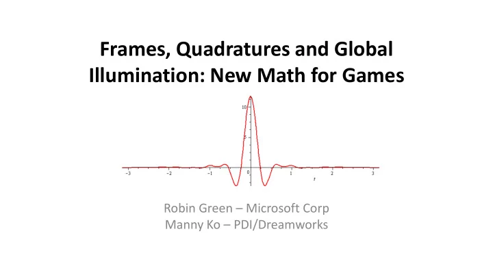
Frames, Quadratures and Global Illumination: New Math for Games Robin Green Microsoft Corp Manny Ko PDI/Dreamworks WARNING This talk is MATH HEAVY We assume you understand the basics of: Linear Algebra, Calculus, 3D Mathematics


  1. Frames, Quadratures and Global Illumination: New Math for Games Robin Green – Microsoft Corp Manny Ko – PDI/Dreamworks

  2. WARNING • This talk is MATH HEAVY • We assume you understand the basics of: – Linear Algebra, Calculus, 3D Mathematics – Spherical Harmonic Lighting, Visibility, BRDF, Cosine Term – Monte Carlo Integration, Unbiased Spherical Sampling – Precomputed Radiance Transfer, Rendering Equation • This is bleeding edge research (like new results last night ) • There are still a lot of unanswered questions

  3. Some Definitions 𝕋 2 is the unit sphere in ℝ 3 • 𝜊 is a point on the sphere • 𝜊 = 𝜄, 𝜒 where 𝜄 ∈ 0,2𝜌 φ ∈ 0, 𝜌 𝜊 = 𝑦, 𝑧, 𝑨 where 𝑦 2 + 𝑧 2 + 𝑨 2 = 1 • Right-handed coordinate system, + z is up

  4. Spherical Harmonics • The Real SH functions are a family of orthonormal basis function on the sphere.

  5. Spherical Harmonics • They are defined on the sphere as a signed function of every direction 𝑛 cos 𝑛𝜒 𝑄 𝑚 𝑛 cos 𝜄 , 2𝐿 𝑚 𝑛 > 0 𝑛 𝜄, 𝜒 = 𝑛 sin −𝑛𝜒 𝑄 𝑚 −𝑛 cos 𝜄 , 𝑧 𝑚 2𝐿 𝑚 𝑛 < 0 0 cos 𝜄 , 0 𝑄 𝑚 𝐿 𝑚 𝑛 = 0 • The functions are orthogonal to each other 𝑧 𝑗 𝜊 𝑧 𝑘 𝜊 ⅆ𝜊 = 𝜀 𝑗𝑘 = 1, 𝑗 = 𝑘 0, i ≠ 𝑘 𝜊∈𝕋 2

  6. SH Deficiencies • SH produces signed values yet all visibility functions, BRDFs and light probes are strictly positive. • SH projections are global and smooth, visibility functions are local and sharp. • SH reproduces a signal at the limit . There is no guarantee the result is close to the original at low orders. Even at high orders it “rings” esp when restricted to the hemisphere.

  7. Haar Wavelets • Haar wavelets are spatially compact and produce a lot of zero coefficients. • Generating 6 times the coefficients, papers rely on compression and highly conditional code. • Projecting cube faces onto the sphere introduces distortions, and seams for filtering and rotation.

  8. Radial Basis Functions • Radial Basis Functions are also used, usually sums of Gaussian lobes. • Need to solve two variables – direction and spread. Leads to conditional code that is not GPU friendly. • Zonal Harmonics are another form of steerable RBF built out of orthogonal parts.

  9. Smoothness vs. Localization • Haar and SH are two ends of a continuum – one smooth and global, the other highly local and unsmooth. This is Spatial vs. Spectral compactness. Q: What lives in the middle ground?

  10. Spatial vs. Spectral • It turns out, the Spatial vs. Spectral problem is exactly Heisenberg’s Uncertainty Principle . • You cannot have both spatial compactness and spectral compactness at the same time – e.g. The Fourier transform of a delta function is infinitely spread out spectrally. • But… thanks to a theorem by David Slepian called the Spherical Concentration Problem you can get pretty close.

  11. Fundamental Questions 1. Where do these Orthonormal Basis Functions come from? 2. How can we loosen the rules so we can define better functions for our own use cases? 3. What are the key properties we need to retain for our functions to be useful?

  12. What You Need To Know • We are going to introduce Frame Theory and Spherical Quadrature , just enough to understand two key concepts: Parseval Tight Frames Spherical t-Designs

  13. Back to Fundamentals We choose a vector space, like ℝ 𝑜 or ℂ 𝑜 • 𝑦 = 𝑦 1 , 𝑦 2 , … , 𝑦 𝑜 where 𝐽 = 1, … , 𝑜 is an index set, we say the space has a dimension 𝑜 • Using the rules of Arithmetic we can add and subtract vectors, or multiply and rescale them using a Scalar value: 𝑦 + 𝑧 = 𝑦 1 + 𝑧 1 , 𝑦 2 + 𝑧 2 , … 𝑦 𝑜 + 𝑧 𝑜 3𝑦 = 3𝑦 1 , 3𝑦 2 , … 3𝑦 𝑜

  14. Back to Fundamentals • When we add an Inner Product and a Norm things get interesting: ∗ 𝑧 𝑗 𝑦, 𝑧 = 𝑦 𝑗 𝑗∈𝐽 𝑦 = 𝑦, 𝑦 • Now we can measure angles, perpendicularity, sizes, distance and similarity: 𝑦, 𝑧 = 0 ⇒ 𝑦 ⊥ 𝑧 • All of Geometry comes from these simple definitions

  15. Hilbert Spaces A Hilbert space ℋ is a vector space with a finite energy • 𝑓 𝑗 , 𝑓 𝑗 < ∞ 𝑗∈ℋ These finite square summable signals termed 𝑀 2 after Lebesgue • 𝑀 2 is the mathematical world of data we see in the real world • – Photographs – Audio streams – Motion Capture or GPS data

  16. Hilbert Spaces The field ℂ has the inner product 𝑦𝑧 • 𝑜 The field ℝ n has the dot product defined 𝑦 𝑗 𝑧 𝑗 • 𝑗=1 The infinite dimensional space of finite sequences ℓ 2 ℕ has the • ∞ inner product 𝑦 𝑗 𝑧 𝑗 𝑗=1 The space of functions on the interval 𝑏, 𝑐 called 𝑀 2 𝑏, 𝑐 has the • standard inner product: 𝑐 𝑔, 𝑕 = 𝑔 𝑦 𝑕 𝑦 ⅆ𝑦 𝑏

  17. Orthonormal Basis An orthonormal basis Φ for Hilbert space ℋ is a set of vectors: • Φ = 𝑓 𝑗 𝑗∈ℤ where each pair of vectors are mutually orthogonal: 𝑓 𝑘 , 𝑓 𝑙 = 𝜀 𝑘,𝑙 span Φ = ℋ – A span(𝑦) is the set of all finite linear combinations of the elements of 𝑦

  18. Orthonormal Bases • For example 2𝜌 𝑓 𝑗𝑜𝑦 𝑜∈ℤ is an orthonormal basis for 𝑀 2 −𝜌, 𝜌 called 1 – the family the standard Fourier basis from which we get the Fourier transform. 1.571 3.142 3.142 x 1.571

  19. Orthonormal Bases • For example – The family of polynomials 1, 𝑦, 𝑦 2 − 1 3 , 𝑦 3 − 3 5 𝑦, … are the Legendre Polynomials , and form an orthonormal basis on the interval 𝑀 2 −1,1 1 1 1 x 1

  20. Orthonormal Bases • For example is an orthonormal basis on ℓ 2 ℕ where ∞ – The family 𝑓 𝑜 𝑜=1 𝑓 1 = 1,0,0,0,0,0,0, … 𝑓 2 = 0,1,0,0,0,0,0, … 𝑓 3 = 0,0,1,0,0,0,0, … – ℓ 2 ℕ is the infinite dimensional space of finite, time-related signals like audio, motion capture joints or accelerometer data.

  21. Orthonormal Basis Characteristics Projection: Given a signal or function 𝑔 ∈ ℋ • 𝑑 𝑗 = 𝑓 𝑗 , 𝑔 If 𝑓 𝑗 is a vector, this projection is a dot product. • 𝑐 If 𝑓 𝑗 is a function in 1D this is an integral 𝑓 𝑗 𝑦 𝑔 𝑦 ⅆ𝑦 𝑏 If 𝑓 𝑗 is a function on the sphere, this integral is over the sphere 𝕋 2𝜌 𝜌 𝑓 𝑗 𝜄, 𝜒 𝑔 𝜄, 𝜒 sin 𝜒 ⅆ𝜄 ⅆ𝜒 𝜒=0 𝜄=0

  22. Orthonormal Basis Characteristics • Perfect reconstruction : 𝑔 = 𝑓 𝑗 , 𝑔 𝑓 𝑗 for all 𝑔 ∈ ℋ 𝑗∈𝐽 • This says we can project then exactly reconstruct our signal from just it’s coefficients

  23. Orthonormal Basis Characteristics • Parseval’s Identity: 𝑔 2 = 𝑓 𝑗 , 𝑔 2 for all 𝑔 ∈ ℋ 𝑗∈𝐽 • Sometimes called norm preservation , this says that the total energy in the function is the same as the magnitude of the coefficients. – This is a key property for a lot of algorithms. Working on coefficients is a lot quicker than working on functions.

  24. ONB Characteristics • Successive Approximation: 𝑙 + 𝑓 𝑙+1 , 𝑦 𝑓 𝑙+1 𝑙+1 = 𝑦 𝑦 • This is a roundabout way of saying that projecting to a subset of indexes is the best approximation in a least squares sense .

  25. General Bases • We use Orthonormal Bases all the time • Every rotation matrix in 3D is an Orthonormal Basis

  26. General Bases • What if you chose vectors that are not orthogonal? Φ = 𝑓 1 , 𝑓 2 𝑓 1 = 1 0 2 2 𝑓 2 = 2 2

  27. General Base • We can still represent points, but we need a “helper” basis to get us there. = 𝑓 1 , 𝑓 2 Φ 1 𝑓 1 = −1 0 𝑓 2 = 2

  28. General Bases We can now project the point 𝑔 = 1 • 1 2 𝑔′ = 𝑓 𝑗 , 𝑔 𝑓 𝑗 𝑗=1 = 𝑓 1 , 𝑔 𝑓 1 + 𝑓 2 , 𝑔 𝑓 2 = 1 ∙ 1 + −1 ∙ 1 𝑓 1 + 0 ∙ 1 + 2 ∙ 1 𝑓 2 = 0 ∙ 𝑓 1 + 2 ∙ 𝑓 2 0 = 2

  29. Biorthogonal Bases • This second “helper” matrix is called the dual basis Φ 𝑓 1 , 𝑓 1 = 1 ∙ 1 + 0 ∙ −1 = 1 2 2 𝑓 2 , 𝑓 2 = 2 ∙ 0 + 2 ∙ 2 = 1 𝑓 𝑘 , 𝑓 𝑙 = 𝜀 𝑘−𝑙 𝑥ℎ𝑓𝑠𝑓 𝜀 = • Biorthogonal bases are pairwise orthogonal and commute. 𝑔 = 𝑓 𝑗 , 𝑔 𝑓 𝑗 = 𝑓 𝑗 , 𝑔 𝑓 𝑗 𝑗∈𝐽 𝑗∈𝐽

  30. Matrix Notation • Now we switch to a matrix Φ = 𝑓 1 , 𝑓 2 , 𝑓 3 , … notation. 𝑓 1𝑦 𝑓 1𝑧 • Every basis in ℋ can be written 𝑓 2𝑦 𝑓 2𝑧 = as a matrix with basis vectors as columns ⋮ ⋮ 𝑞 = 𝑦 𝑧 • Points are now column vectors.

  31. Matrix Notation • Our projection and reconstruction now turn into operators 𝑔 𝑞 = Φ 𝑔 = Φ ∗ 𝑞 (where 𝑁 ∗ is the transpose) • We can now show that orthonormal bases are self dual : = Φ Φ Φ ∗ = I Φ

  32. Breaking the Rules • What happens if we add another vector to the basis? = 𝑓 1 , 𝑓 2 , 𝑓 3 Φ = 𝑓 1 , 𝑓 2 , 𝑓 3 Φ 1 0 2 0 = 0 1 = −1 1 1 −1 −1 0 • Now we have an overcomplete system , and coordinates are now linearly dependent

  33. Breaking the Rules = 𝑓 𝑗 𝑗∈𝐽 Φ = 𝑓 𝑗 𝑗∈𝐽 Φ

Download Presentation
Download Policy: The content available on the website is offered to you 'AS IS' for your personal information and use only. It cannot be commercialized, licensed, or distributed on other websites without prior consent from the author. To download a presentation, simply click this link. If you encounter any difficulties during the download process, it's possible that the publisher has removed the file from their server.

Recommend


More recommend