1 Reflection Equation Reflection Equation i i r r x x - PDF document

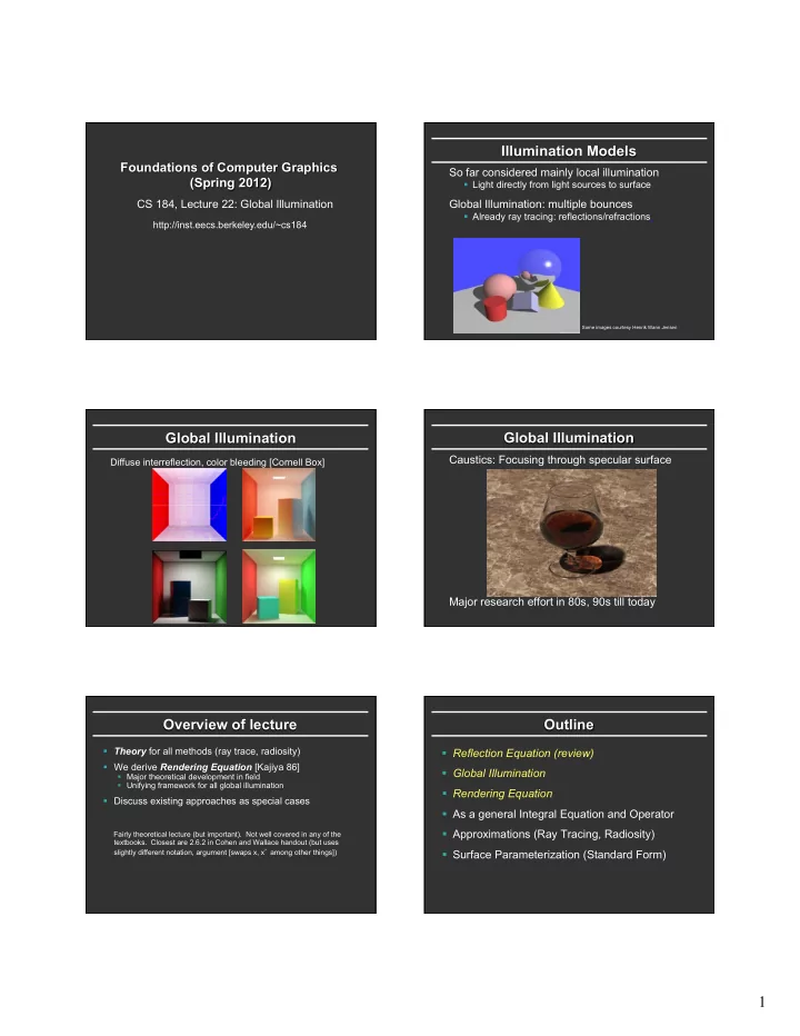
Illumination Models Foundations of Computer Graphics So far considered mainly local illumination (Spring 2012)  Light directly from light sources to surface CS 184, Lecture 22: Global Illumination Global Illumination: multiple bounces  Already ray tracing: reflections/refractions http://inst.eecs.berkeley.edu/~cs184 Some images courtesy Henrik Wann Jensen Global Illumination Global Illumination Caustics: Focusing through specular surface Diffuse interreflection, color bleeding [Cornell Box] Major research effort in 80s, 90s till today Overview of lecture Outline  Theory for all methods (ray trace, radiosity)  Reflection Equation (review)  We derive Rendering Equation [Kajiya 86]  Global Illumination  Major theoretical development in field  Unifying framework for all global illumination  Rendering Equation  Discuss existing approaches as special cases  As a general Integral Equation and Operator  Approximations (Ray Tracing, Radiosity) Fairly theoretical lecture (but important). Not well covered in any of the textbooks. Closest are 2.6.2 in Cohen and Wallace handout (but uses slightly different notation, argument [swaps x, x ’ among other things])  Surface Parameterization (Standard Form) 1

Reflection Equation Reflection Equation ω i ω i ω ω r r x x Sum over all light sources L r ( x , ω r ) = L e ( x , ω r ) + ∑ L i ( x , ω i ) f ( x , ω i , ω r )( ω i i n ) L r ( x , ω r ) = L e ( x , ω r ) + L i ( x , ω i ) f ( x , ω i , ω r )( ω i i n ) Cosine of Cosine of Reflected Light Emission Incident BRDF Reflected Light Emission Incident BRDF (Output Image) Light (from Incident angle (Output Image) Light (from Incident angle light source) light source) Reflection Equation Global Illumination Surfaces (interreflection) ′ x dA ω i ω i d ω ω d ω ω r i i r x x ω i  x − x ′ Replace sum with integral + ∫ ∫ L r ( ′ L x ( , ω ) = L x ( , ω ) L x ( , ω ) ( , f x ω , ω ) cos θ d ω L r ( x , ω r ) = L e ( x , ω r ) + x , − ω i ) f ( x , ω i , ω r ) cos θ i d ω i r r e r i i i r i i Ω Ω Cosine of Cosine of Reflected Light Emission Incident BRDF Reflected Light Emission Reflected BRDF (Output Image) Incident angle (Output Image) Incident angle Light (from Light (from light source) surface) Rendering Equation Rendering Equation (Kajiya 86) Surfaces (interreflection) ′ x dA ω i d ω ω i r x ∫ L r ( ′ L r ( x , ω r ) = L e ( x , ω r ) + x , − ω i ) f ( x , ω i , ω r ) cos θ i d ω i Ω Reflected Light Emission Reflected BRDF Cosine of Incident angle (Output Image) Light UNKNOWN KNOWN UNKNOWN KNOWN KNOWN 2

Rendering Equation as Integral Equation Outline ∫ L r ( ′ L r ( x , ω r ) = L e ( x , ω r ) + x , − ω i ) f ( x , ω i , ω r ) cos θ i d ω i  Reflectance Equation (review) Ω Cosine of Reflected Light Emission Reflected BRDF  Global Illumination (Output Image ) Incident angle Light UNKNOWN KNOWN KNOWN  Rendering Equation UNKNOWN KNOWN  As a general Integral Equation and Operator Is a Fredholm Integral Equation of second kind [extensively studied numerically] with canonical form  Approximations (Ray Tracing, Radiosity) ∫ l ( u ) = e ( u ) + l ( v ) K ( u , v ) dv  Surface Parameterization (Standard Form) The material in this part of the lecture is fairly advanced and Kernel of equation not covered in any of the texts. The slides should be fairly complete. This section is fairly short, and I hope some of you will get some insight into solutions for general global illumination Linear Operator Equation Solution Techniques All global illumination methods try to solve + ∫ = l u ( ) e u ( ) l v ( ) K u ( , ) v dv (approximations of) the rendering equation – Too hard for analytic solution: numerical methods Kernel of equation – General theory of solving integral equations Light Transport Operator L = E + KL Radiosity (next lecture; usually diffuse surfaces) – General class numerical finite element methods (divide surfaces in scene into a finite set elements or patches) Can be discretized to a simple matrix equation – Set up linear system (matrix) of simultaneous equations [or system of simultaneous linear equations] – Solve iteratively (L, E are vectors, K is the light transport matrix) Ray Tracing and extensions Ray Tracing L = E + KE + K 2 E + K 3 E + ... – General class numerical Monte Carlo methods – Approximate set of all paths of light in scene L = E + KL Emission directly From light sources IL − KL = E ( I − K ) L = E Direct Illumination on surfaces L = ( I − K ) − 1 E Global Illumination Binomial Theorem (One bounce indirect) L = ( I + K + K 2 + K 3 + ...) E [Mirrors, Refraction] (Two bounce indirect) L = E + KE + K 2 E + K 3 E + ... [Caustics etc] 3

Ray Tracing Outline L = E + KE + K 2 E + K 3 E + ...  Reflectance Equation (review)  Global Illumination Emission directly  Rendering Equation From light sources  As a general Integral Equation and Operator Direct Illumination on surfaces  Approximations (Ray Tracing, Radiosity) Global Illumination OpenGL Shading  Surface Parameterization (Standard Form) (One bounce indirect) [Mirrors, Refraction] (Two bounce indirect) [Caustics etc] Rendering Equation Change of Variables Surfaces (interreflection) ∫ ω = ω + ′ − ω ω ω θ ω L x ( , ) L x ( , ) L x ( , ) ( , f x , ) cos d ′ x r r e r r i i r i i Ω dA Integral over angles sometimes insufficient. Write integral in terms of surface radiance only (change of variables) ω i d ω i ω r ′ x θ o x d ′ A ω i  x − x ′ − ω i d ω i = d ′ A cos θ o d ω i ∫ L r ( ′ L r ( x , ω r ) = L e ( x , ω r ) + x , − ω i ) f ( x , ω i , ω r ) cos θ i d ω i θ i ω i | x − ′ x | 2 Ω Cosine of Reflected Light Emission Reflected BRDF x (Output Image) Incident angle Light UNKNOWN KNOWN KNOWN UNKNOWN KNOWN Change of Variables Rendering Equation: Standard Form ∫ ∫ ω = ω + ′ − ω ω ω θ ω ω = ω + ′ − ω ω ω θ ω L x ( , ) L x ( , ) L x ( , ) ( , f x , ) cos d L x ( , ) L x ( , ) L x ( , ) ( , f x , ) cos d r r e r r i i r i i r r e r r i i r i i Ω Ω Integral over angles sometimes insufficient. Write integral Integral over angles sometimes insufficient. Write integral in terms of surface radiance only (change of variables) in terms of surface radiance only (change of variables) θ θ θ θ cos cos cos cos ∫ ′ ′ ∫ ′ ′ L x ( , ω ) = L x ( , ω ) + L x ( , − ω ) ( , f x ω ω , ) i o d A L x ( , ω ) = L x ( , ω ) + L x ( , − ω ) ( , f x ω ω , ) i o d A r r e r r i i r − ′ 2 r r e r r i i r − ′ 2 | x x | | x x | ′ ′ all x visible to x all x visible to x Domain integral awkward. Introduce binary visibility fn V ∫ ω = ω + ′ − ω ω ω ′ ′ ′ L x ( , ) L x ( , ) L x ( , ) ( , f x , ) ( , G x x V ) ( , x x ) dA r r e r r i i r ′ all surfaces x d ω i = d ′ A cos θ o d ω i = d ′ A cos θ o Same as equation 2.52 Cohen Wallace. It swaps primed | x − ′ | x − ′ x | 2 x | 2 And unprimed, omits angular args of BRDF, - sign. x , x ) = cos θ i cos θ o x , x ) = cos θ i cos θ o G ( x , ′ x ) = G ( ′ G ( x , ′ x ) = G ( ′ | x − ′ x | 2 | x − ′ x | 2 4

Overview  Theory for all methods (ray trace, radiosity)  We derive Rendering Equation [Kajiya 86]  Major theoretical development in field  Unifying framework for all global illumination  Discuss existing approaches as special cases 5