forming an image
play

Forming an Image Illuminate the surface to get: Learning to - PDF document

Forming an Image Illuminate the surface to get: Learning to separate shading from paint Marshall F. Tappen 1 William T. Freeman 1 Edward H. Adelson 1,2 Surface Shading Image 1 MIT Computer Science and Artificial Intelligence Laboratory (CSAIL)


  1. Forming an Image Illuminate the surface to get: Learning to separate shading from paint Marshall F. Tappen 1 William T. Freeman 1 Edward H. Adelson 1,2 Surface Shading Image 1 MIT Computer Science and Artificial Intelligence Laboratory (CSAIL) The “shading image” is the interaction of the shape of the surface and the illumination 2 MIT Dept. of Brain and Cognitive Sciences Marshall
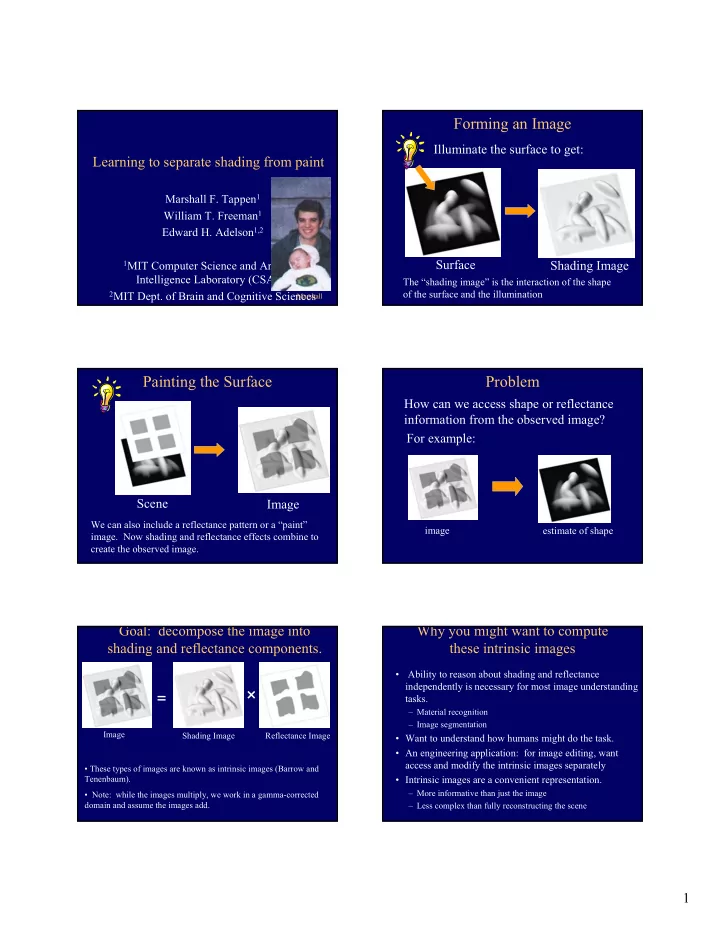
 Painting the Surface Problem How can we access shape or reflectance information from the observed image? For example: Scene Image We can also include a reflectance pattern or a “paint” image estimate of shape image. Now shading and reflectance effects combine to create the observed image. Goal: decompose the image into Why you might want to compute shading and reflectance components. these intrinsic images • Ability to reason about shading and reflectance independently is necessary for most image understanding � = tasks. – Material recognition – Image segmentation Image Shading Image Reflectance Image • Want to understand how humans might do the task. • An engineering application: for image editing, want access and modify the intrinsic images separately • These types of images are known as intrinsic images (Barrow and Tenenbaum). • Intrinsic images are a convenient representation. – More informative than just the image • Note: while the images multiply, we work in a gamma-corrected domain and assume the images add. – Less complex than fully reconstructing the scene 1

  2. Recovering Intrinsic Images Treat the separation as a labeling problem • Classify each x and y image derivative as being caused by either shading or a reflectance change • We want to identify what parts of the image • Recover the intrinsic images by finding the least- were caused by shape changes and what squares reconstruction from each set of labeled parts were caused by paint changes. derivatives. (Fast Matlab code for that available • But how represent that? Can’t label pixels from Yair Weiss’s web page.) of the image as “shading” or “paint”. • Solution: we’ll label gradients in the image as being caused by shading or paint. • Assume that image gradients have only one cause. Classify each derivative Original x derivative image (White is reflectance) Outline of our algorithm Classic algorithm: Retinex (and the rest of the talk) • Gather local evidence for shading or reflectance – Color (chromaticity changes) – Form (local image patterns) • Integrate the local evidence across space. • Assume world is made up of Mondrian reflectance – Assume a probabilistic model and use belief patterns and smooth illumination propagation. • Can classify derivatives by the magnitude of the • Show results on example images derivative Probabilistic graphical model Probabilistic graphical model • Local evidence Local Color Evidence Unknown Some statistical relationship that Derivative Labels Derivative Labels (hidden random we’ll specify variables that we want to estimate) 2

  3. Probabilistic graphical model Probabilistic graphical model • Local evidence Propagate the local evidence in Markov Random Field. This strategy can be used to solve other low-level vision problems. Local Evidence Local Form Evidence Local Color Evidence Hidden state to be Derivative Labels estimated Influence of Neighbor Local Color Evidence Classifying Color Changes Chromaticity Changes Intensity Changes For a Lambertian surface, and simple illumination conditions, shading only Angle between Angle between affects the intensity of the color of a the two vectors, two vectors, θ , θ , is greater surface equals 0 than 0 Red Red e e Notice that the chromaticity of each face is the u u l l B B θ same Any change in chromaticity must be a reflectance change Green Green Color Classification Algorithm Result using only color information 1. Normalize the two color vectors c 1 and c 2 c 1 c 2 2. If ( c 1 � c 2 ) > T • Derivative is a reflectance change • Otherwise, label derivative as shading 3

  4. Results Using Only Color Utilizing local intensity patterns • The painted eye and the ripples of the fabric have very different appearances Input Reflectance Shading • Can learn classifiers • Some changes are ambiguous which take advantage • Intensity changes could be caused by shading or reflectance of these differences – So we label it as “ambiguous” – Need more information From Weak to Strong Classifiers: Shading/paint training set Boosting Examples from Reflectance Change Training Set • Individually these weak classifiers aren’t very good. • Can be combined into a single strong classifier. • Call the classification from a weak classifier h i (x). • Each h i (x) votes for the classification of x (-1 or 1). • Those votes are weighted and combined to produce a Examples from Shading Training Set final classification. ⎛ ⎞ ∑ = α ⎜ ⎟ H ( x ) sign h ( x ) i i ⎝ ⎠ i Using Local Intensity Patterns AdaBoost Initial uniform weight on training examples (Freund & Shapire ’95) ⎛ ⎞ ∑ = θ ⎜ α ⎟ • Create a set of weak classifiers that use a f ( x ) h ( x ) weak classifier 1 t t ⎝ ⎠ t small image patch to classify each derivative ⎛ ⎞ error Incorrect classifications ⎜ ⎟ α = 0 . 5 log t re-weighted more heavily ⎜ ⎟ t − • The classification of a derivative: 1 error ⎝ ⎠ t weak classifier 2 − α i y h ( x ) w e i t t i w i = t − 1 ∑ > T t − α w i e y h ( x ) i t t i t − 1 � abs i weak classifier 3 Final classifier is weighted F combination of weak classifiers I p Viola and Jones, Robust object detection using a boosted cascade of simple features, CVPR 2001 4

  5. Use Newton’s method to reduce Adaboost demo… classification cost over training set ∑ = − y f ( x ) Classification cost J e i i i Treat h m as a perturbation, and expand loss J to second order in h m cost classifier with squared error function perturbation reweighting Learning the Classifiers Classifiers Chosen • The weak classifiers, h i (x) , and the weights α are chosen using the AdaBoost algorithm (see www.boosting.org for introduction). • Train on synthetic images. • Assume the light direction is from the right. • These are the filters chosen for classifying • Filters for the candidate weak classifiers—cascade two out of these 4 categories: vertical derivatives when the illumination – Multiple orientations of 1 st derivative of Gaussian filters comes from the top of the image. – Multiple orientations of 2 nd derivative of Gaussian filters – Several widths of Gaussian filters • Each filter corresponds to one h i (x) – impulse Characterizing the learned Results Using Only classifiers Form Information • Learned rules for all (but classifier 9) are: if rectified filter response is above a threshold, vote for reflectance. • Yes, contrast and scale are all folded into that. We perform an Reflectance Image Input Image Shading Image overall contrast normalization on all images. • Classifier 1 (the best performing single filter to apply) is an empirical justification for Retinex algorithm: treat small derivative values as shading. • The other classifiers look for image structure oriented perpendicular to lighting direction as evidence for reflectance change. 5

  6. Some Areas of the Image Are Using Both Color and Locally Ambiguous Form Information Is the change here better explained as Input image Shading Reflectance Input ? or Results only using chromaticity. Reflectance Shading Propagating Information Markov Random Fields • Can disambiguate areas by propagating information from reliable areas of the image • Allows rich probabilistic models for into ambiguous areas of the image images. • But built in a local, modular way. Learn local relationships, get global effects out. Network joint probability Inference in MRF’s • Inference in MRF’s. (given observations, how infer the hidden states?) 1 ∏ ∏ = Ψ Φ P ( x , y ) ( x , x ) ( x , y ) – Gibbs sampling, simulated annealing i j i i Z – Iterated condtional modes (ICM) i , j i – Variational methods scene Scene-scene Image-scene – Belief propagation compatibility compatibility image – Graph cuts function function neighboring local scene nodes observations See www.ai.mit.edu/people/wtf/learningvision for a tutorial on learning and vision. 6

Download Presentation
Download Policy: The content available on the website is offered to you 'AS IS' for your personal information and use only. It cannot be commercialized, licensed, or distributed on other websites without prior consent from the author. To download a presentation, simply click this link. If you encounter any difficulties during the download process, it's possible that the publisher has removed the file from their server.

Recommend


More recommend