SLIDE 1
Floquet Theory for Internal Gravity Waves in a Density-Stratified Fluid
Yuanxun Bill Bao Senior Supervisor: Professor David J. Muraki August 3, 2012
SLIDE 2
Density-Stratified Fluid Dynamics
Density-Stratified Fluids ⊲ density of the fluid varies with altitude
⊲ stable stratification: heavy fluids below light fluids, internal waves ⊲ unstable stratification: heavy fluids above light fluids, convective dynamics
Buoyancy-Gravity Restoring Dynamics ⊲ uniform stable stratification: dρ/dz < 0 constant ⊲ vertical displacements ⇒ oscillatory motions
SLIDE 3
Internal Gravity Waves
⊲ evidence of internal gravity waves in the atmosphere
⊲ left: lenticular clouds near Mt. Ranier, Washington ⊲ right: uniform flow over a mountain ⇒ oscillatory wave motions
⊲ scientific significance of studying internal gravity waves
⊲ internal waves are known to be unstable ⊲ a major suspect of clear-air-turbulence
SLIDE 4
Gravity Wave Instability: Three Approaches
Triad resonant instability (Davis & Acrivos 1967, Hasselmann 1967) ⊲ primary wave + 2 infinitesimal disturbances ⇒ exponential growth ⊲ perturbation analysis Direct Numerical Simulation (Lin 2000) ⊲ primary wave + weak white-noise modes ⊲ stability diagram
⊲ unstable Fourier modes
Linear Stability Analysis & Floquet-Fourier method (Mied 1976, Drazin 1977) ⊲ linearized Boussinesq equations & stability via eigenvalue computation
SLIDE 5
My Thesis Goal
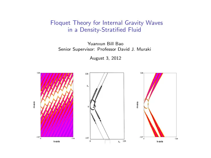
⊲ Floquet-Fourier computation: over-counting of instability in wavenumber space ⊲ Lin’s DNS: two branches of disturbance Fourier modes ⊲ goal: to identify all physically unstable modes from Floquet-Fourier computation
SLIDE 6
My Thesis Goal
⊲ Floquet-Fourier computation: over-counting of instability in wavenumber space ⊲ Lin’s DNS: two branches of disturbance Fourier modes ⊲ goal: to identify all physically unstable modes from Floquet-Fourier computation
SLIDE 7 The Governing Equations
Boussinesq Equations in Vorticity-Buoyancy Form ∇ · u = ; Dη Dt = −bx ; Db Dt = −N 2w ⊲ incompressible, inviscid Boussinesq Fluid
⊲ Euler equations + weak density variation (the Boussinesq approximation) ⊲ Brunt-Vaisala frequency N: uniform stable stratification, N 2 > 0
⊲ 2D velocity: u(x, z, t) ; buoyancy: b(x, z, t)
⊲ streamfunction:
u = u w
∇ × ψ ˆ y = −ψz ψx
∇ × u = η ˆ y = ∇2ψ ˆ y
SLIDE 8 Exact Plane Gravity Wave Solutions +
z y x
−
buoyancy b
Dη Dt = −bx
− + +
buoyancy b
−
Db Dt = −N 2w ⊲ dynamics of buoyancy & vorticity ⇒ oscillatory wave motions ⊲ exact plane gravity wave solutions ψ b η = −Ωd/K N 2 N 2K/Ωd 2A sin(Kx + Mz − Ωdt)
⊲ primary wavenumbers: (K, M) ⊲ dispersion relation: Ω2 d(K, M) =
N 2K2 K2 + M2 .
SLIDE 9 Linear Stability Analysis
⊲ dimensionless exact plane wave + small disturbances ψ b η = −Ω 1 1/Ω 2ǫ sin(x + z − Ωt) + ˜ ψ ˜ b ˜ η
⊲ ǫ: dimensionless amplitude & dimensionless frequency: Ω2 =
1 1 + δ2 ⊲ linearized Boussinesq equations δ2 ˜ ψxx + ˜ ψzz = ˜ η ˜ ηt + ˜ bx − 2ǫJ( Ω˜ η + ˜ ψ/Ω , sin(x + z − Ωt) ) = ˜ bt − ˜ ψx − 2ǫJ( Ω˜ b + ˜ ψ , sin(x + z − Ωt) ) =
⊲ δ = K/M: related to the wave propagation angle (Lin: δ = 1.7) ⊲ Jacobian determinant
J(f, g) =
gx fz gz
fxgz − gxfz
SLIDE 10
Linear Stability Analysis
⊲ dimensionless exact plane wave + small disturbances ψ b η = −Ω 1 1/Ω 2ǫ sin(x + z − Ωt) + ˜ ψ ˜ b ˜ η
⊲ ǫ: dimensionless amplitude & dimensionless frequency: Ω2 =
1 1 + δ2 ⊲ linearized Boussinesq equations δ2 ˜ ψxx + ˜ ψzz = ˜ η ˜ ηt + ˜ bx − 2ǫJ( Ω˜ η + ˜ ψ/Ω , sin(x + z − Ωt) ) = ˜ bt − ˜ ψx − 2ǫJ( Ω˜ b + ˜ ψ , sin(x + z − Ωt) ) =
⊲ system of linear PDEs with non-constant, but periodic coefficients ⊲ analyzed by Floquet theory ⊲ classical textbook example: Mathieu equation (Chapter 3)
SLIDE 11 Floquet Theory: Mathieu Equation
Mathieu Equation: d2u dt2 +
⊲ second-order linear ODE with periodic coefficients ⊲ Floquet theory: u = e−iωt · p(t) = exponential part × co-periodic part ⊲ Floquet exponent ω(k; ǫ): Im ω > 0 → instability ⊲ goal: to identify all unstable solutions in (k, ǫ)-space
SLIDE 12 Floquet Theory: Mathieu Equation
Mathieu Equation: d2u dt2 +
Two perspectives: ⊲ perturbation analysis ⇒ two branches of Floquet exponent
⊲ away from resonances: ω(k; ǫ) ∼ ±k ⊲ resonant instability at primary resonance
2
2 + i ǫ ⊲ Floquet-Fourier computation of ω(k; ǫ)
⊲ a Riemann surface interpretation of ω(k; ǫ) with k ∈ C
SLIDE 13 Floquet-Fourier Computation
⊲ Mathieu equation in system form: d dt u v
i
k2 − 2ǫ cos(t) u v
Floquet-Fourier representation: u v
∞
⊲ ω(k; ǫ) as eigenvalues of Hill’s bi-infinite matrix:
... ... ... S0 ǫM ǫM S1 ... ... ... ⊲ 2 × 2 real blocks: Sm and M
⊲ truncated Hill’s matrix: −N ≤ m ≤ N
⊲ real-coefficient characteristic polynomial ⊲ compute 4N + 2 eigenvalues: {ωn(k; ǫ)}
⊲ ǫ = 0, eigenvalues from Sn blocks: ωn(k; 0) = −n ± k & all real-valued ⊲ ǫ ≪ 1, complex eigenvalues may arise from ǫ = 0 double eigenvalues
SLIDE 14 Floquet-Fourier Computation
−2 −1.5 −1 −0.5 0.5 1 1.5 2 −2 −1.5 −1 −0.5 0.5 1 1.5 2
k−axis Re ω ε = 0.1
⊲ ωn(k; ǫ): real • ; complex • ⊲ ‘——’: ωn(k; 0) = −n ± k ‘——’: ω0(k; 0) = ± k ⊲ ωn(k; ǫ) curves are close to ωn(k; 0) ⊲ two continuous curves close to ±k ⊲ the rest are shifted due to u v
∞
⊲ For each k, how many Floquet exponents are associated with the unstable solu- tions of Mathieu equation? two or ∞? Both!
⊲ two is understood from perturbation analysis ⊲ ∞ will be understood from the Riemann surface of ω(k; ǫ) with k ∈ C
SLIDE 15 Floquet-Fourier Computation
−2 −1 1 2 −2 −1 1 2
k−axis Re ω ε = 0.1
⊲ ωn(k; ǫ): real • ; complex • ⊲ ‘——’: ωn(k; 0) = −n ± k ‘——’: ω0(k; 0) = ± k ⊲ ωn(k; ǫ) curves are close to ωn(k; 0) ⊲ two continuous curves close to ±k ⊲ the rest are shifted due to u v
∞
⊲ For each k, how many Floquet exponents are associated with the unstable solu- tions of Mathieu equation? two or ∞? Both!
⊲ two is understood from perturbation analysis ⊲ ∞ will be understood from the Riemann surface of ω(k; ǫ) with k ∈ C
SLIDE 16 A Riemann Surface Interpretation of ω(k; ǫ)
−2 −1 1 2 −2 −1 1 2
k−axis Re ω ε = 0.1
⊲ Floquet-Fourier computation with k ∈ C → the Riemann surface of ω(k; ǫ)
⊲ surface height: real ω ; surface colour: imag ω ⊲ layers of curves for k ∈ R become layers of sheets for k ∈ C ⊲ the two physical branches belong to two primary Riemann sheets
⊲ How to identify the two primary Riemann sheets?
⊲ more understanding of how sheets are connected
SLIDE 17
A Riemann Surface Interpretation of ω(k; ǫ)
⊲ zoomed view near Re k = 1/2 shows Riemann sheet connection ⊲ branch points: end points of instability intervals
⊲ loop around the branch points ⇒ √ type
⊲ branch cuts coincide with instability intervals (McKean & Trubowitz 1975)
SLIDE 18
A Riemann Surface Interpretation of ω(k; ǫ)
⊲ zoomed view near Re k = 0 shows Riemann sheet connection ⊲ branch points: two on imaginary axis
⊲ loop around the branch points ⇒ √ type
⊲ branch cuts to ± i∞ give V-shaped sheets
SLIDE 19 A Riemann Surface Interpretation of ω(k; ǫ)
−1 −0.5 0.5 1 −i √ 2ǫ i √ 2ǫ real k imag k ε = 0.1
⊲ branch cuts: instability intervals & two cuts to ± i∞ ⊲ two primary sheets: upward & downward V-shaped sheets
⊲ associated with the two physically-relevant Floquet exponents ⊲ the other sheets are integer-shifts of primary sheets
SLIDE 20 A Riemann Surface Interpretation of ω(k; ǫ)
−1 −0.5 0.5 1 −i √ 2ǫ i √ 2ǫ real k imag k ε = 0.1
⊲ branch cuts: instability intervals & two cuts to ± i∞ ⊲ two primary sheets: upward & downward V-shaped sheets
⊲ associated with the two physically-relevant Floquet exponents ⊲ the other sheets are integer-shifts of primary sheets
SLIDE 21 Recap of Mathieu Equation
⊲ Floquet-Fourier:
u v
N
⊲ 4N + 2 computed Floquet exponents ωn(k; ǫ)
⊲ perturbation analysis: ω(k; ǫ) ∼ ±k ⊲ Riemann surface has two primary Riemann sheets (physically-relevant)
−2 −1 1 2 −2 −1 1 2
k−axis Re ω ε = 0.1
SLIDE 22 Chapter 4, 5, 6 of My Thesis
⊲ Floquet-Fourier:
ψ ˜ b
N
ψ n ˆ b n
. ⊲ 4N + 2 computed Floquet exponents ωn(k, m; ǫ, δ)
⊲ perturbation analysis: ω(k, m; ǫ, δ) ∼ ±
|k|
√
δ2k2+m2
⊲ Riemann surface analysis ⇒ physically-relevant Floquet exponents
−2 −1 1 2 −2 −1 1 2
k−axis, (k−m = 2.5) real ω ε = 0.1, δ = 1.7
SLIDE 23 Gravity Wave Stability Problem
⊲ four parameters of ω(k, m; ǫ, δ)
⊲ ǫ, δ = 1.7 (Lin) ⊲ wavevector, (k, m) ;
k ∈ C with k − m = 2.5 ⊲
- ver-counting of Floquet-Fourier computation
⊲ vertical & horizontal shifts
→ instability bands
−2 −1 1 2 −2 −1 1 2
k−axis, (k−m = 2.5) real ω ε = 0.1, δ = 1.7
SLIDE 24 Gravity Wave Stability Problem
⊲ four parameters of ω(k, m; ǫ, δ)
⊲ ǫ, δ = 1.7 (Lin) ⊲ wavevector, (k, m) ;
k ∈ C with k − m = 2.5 ⊲
- ver-counting of Floquet-Fourier computation
⊲ vertical & horizontal shifts
→ instability bands
−2 −1 1 2 −2 −1 1 2
k−axis, (k−m = 2.5) real ω ε = 0.1, δ = 1.7
⊲ physically-relevant Floquet exponents solves over-counting problem
SLIDE 25 Fixing the Gap along k − m = 1
−2 −1.5 −1 −0.5 0.5 1 1.5 2 −2 −1.5 −1 −0.5 0.5 1 1.5
real−k δ = 1.7, ε = 0.1 real ω
⊲ new feature: four-sheet collision (only two for Mathieu!) ⊲ physically corresponds to near-resonance of four fourier modes (section 5.3)
SLIDE 26 Fixing the Gap along k − m = 1
−0.4 −0.2 0.2 0.4 −0.4 −0.2 0.2 0.4 sheet 4 sheet 2 sheet 1 sheet 3 real k real ω ε = 0.1, δ = 1.7
⊲ zoomed view near Re k = 0 with Riemann surface
SLIDE 27 Fixing the Gap along k − m = 1
−0.4 −0.2 0.2 0.4 −0.4 −0.2 0.2 0.4 sheet 4 sheet 2 sheet 1 sheet 3 real k real ω ε = 0.1, δ = 1.7 −0.4 −0.2 0.2 0.4 −0.4 −0.2 0.2 0.4 ω−(k,m;0) ω−(k+1,m+1;0)−Ω ω+(k,m;0) ω+(k−1,m−1;0)+Ω k−axis ω(k,m) δ = 1.7, ε = 0
⊲ continuation algorithm for ω(k, m; ǫ = 0.1) starts from ǫ = 0 values
SLIDE 28 Fixing the Gap along k − m = 1
−0.4 −0.2 0.2 0.4 −0.4 −0.2 0.2 0.4 sheet 4 sheet 2 sheet 1 sheet 3 real k real ω ε = 0.02, δ = 1.7 −0.4 −0.2 0.2 0.4 −0.4 −0.2 0.2 0.4 ω−(k,m;0) ω−(k+1,m+1;0)−Ω ω+(k,m;0) ω+(k−1,m−1;0)+Ω k−axis ω(k,m) δ = 1.7, ε = 0
⊲ continuation algorithm for ω(k, m; ǫ = 0.1) starts from ǫ = 0 values
⊲ ǫ = 0.02: shows ǫ = 0 limit incorrect
SLIDE 29 Fixing the Gap along k − m = 1
−0.4 −0.2 0.2 0.4 −0.4 −0.2 0.2 0.4 sheet 4 sheet 2 sheet 1 sheet 3 real k real ω ε = 0.02, δ = 1.7 −0.4 −0.2 0.2 0.4 −0.4 −0.2 0.2 0.4 sheet 4 sheet 2 sheet 1 sheet 3 real k real ω ε = 0, δ = 1.7
⊲ continuation algorithm for ω(k, m; ǫ = 0.1) starts from ǫ = 0 values
⊲ ǫ = 0.02: suggests redefining ǫ = 0 branch values (continuous)
SLIDE 30 Fixing the Gap along k − m = 1
−0.4 −0.2 0.2 0.4 −0.4 −0.2 0.2 0.4 sheet 4 sheet 2 sheet 1 sheet 3 real k real ω ε = 0.06, δ = 1.7 −0.4 −0.2 0.2 0.4 −0.4 −0.2 0.2 0.4 sheet 4 sheet 2 sheet 1 sheet 3 real k real ω ε = 0, δ = 1.7
⊲ continuation algorithm for ω(k, m; ǫ = 0.1) starts from ǫ = 0 values
⊲ ǫ = 0.06: instability bands are about to merge
SLIDE 31 Fixing the Gap along k − m = 1
−0.4 −0.2 0.2 0.4 −0.4 −0.2 0.2 0.4 sheet 4 sheet 2 sheet 1 sheet 3 real k real ω ε = 0.1, δ = 1.7 −0.4 −0.2 0.2 0.4 −0.4 −0.2 0.2 0.4 sheet 4 sheet 2 sheet 1 sheet 3 real k real ω ε = 0, δ = 1.7
⊲ continuation algorithm for ω(k, m; ǫ = 0.1) starts from ǫ = 0 values
⊲ ǫ = 0.1: the gap is fixed
SLIDE 32 Instabilities from Two Primary Sheets
⊲ stability diagram is a superposition of instabilities from the two primary sheets ⊲ both primary sheets are continuous in Re ω & Im ω ⊲
- ver-counting problem is solved by complex analysis!
SLIDE 33
In Closing: What I Have Learned
⊲ density-stratified fluid dynamics & internal gravity waves ⊲ linear stability analysis ⊲ the Mathieu equation, Floquet theory & Floquet-Fourier computation ⊲ perturbation analysis (near & away from resonance) ⊲ understanding the Riemann surface structure & computation
SLIDE 34 Four Sheets: ǫ = 0.1
−0.4 −0.2 0.2 0.4 −0.4 −0.2 0.2 0.4 sheet 4 sheet 2 sheet 1 sheet 3 real k real ω ε = 0.1, δ = 1.7
−0.2 −0.1 0.1 0.2 −0.1 −0.05 0.05 0.1
sheet 1
real k imag k ε = 0.1 −0.2 −0.1 0.1 0.2 −0.1 −0.05 0.05 0.1
sheet 2
real k imag k ε = 0.1 −0.2 −0.1 0.1 0.2 −0.1 −0.05 0.05 0.1
sheet 3
real k imag k ε = 0.1 −0.2 −0.1 0.1 0.2 −0.1 −0.05 0.05 0.1
sheet 4
real k imag k ε = 0.1