
SLIDE 1
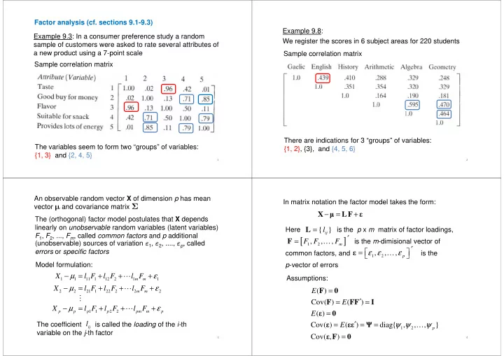
Factor analysis (cf. sections 9.1-9.3) Example 9.3: In a consumer preference study a random sample of customers were asked to rate several attributes of a new product using a 7-point scale Sample correlation matrix
1
The variables seem to form two “groups” of variables: {1, 3} and {2, 4, 5} Example 9.8: We register the scores in 6 subject areas for 220 students Sample correlation matrix
2
There are indications for 3 “groups” of variables: {1, 2}, {3}, and {4, 5, 6} Model formulation: An observable random vector X of dimension p has mean vector and covariance matrix Σ The (orthogonal) factor model postulates that X depends linearly on unobservable random variables (latent variables) F1, F2, ..., Fm, called common factors and p additional (unobservable) sources of variation ε1, ε2, ...., εp, called errors or specific factors
3
Model formulation:
1 1 11 1 12 2 1 1 m m
X l F l F l F µ ε − = + + + ⋯
2 2 21 1 22 2 2 2 m m
X l F l F l F µ ε − = + + + ⋯
1 1 2 2 p p p p pm m p
X l F l F l F µ ε − = + + + ⋯
The coefficient is called the loading of the i-th variable on the j-th factor
ij
l ⋮ − = + X
- LF
ε
In matrix notation the factor model takes the form: Here is the p x m matrix of factor loadings, is the m-dimisional vector of common factors, and is the p-vector of errors
{ }
ij
l = L
[ ]
1 2
, , ,
m
F F F ′ = F …
1 2
, , ,
p
ε ε ε ′ = ε …
4
( ) Cov( ) ( ) E E = ′ = = F F FF I
p-vector of errors Assumptions:
1 2
( ) Cov( ) ( ) diag{ , , , }
p