Linear Algebra Vectors A column vector is a list of numbers stored - - PowerPoint PPT Presentation

Linear Algebra

Vectors

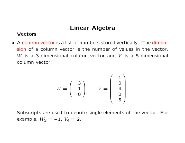
• A column vector is a list of numbers stored vertically. The dimen-

sion of a column vector is the number of values in the vector. W is a 3-dimensional column vector and V is a 5-dimensional column vector: W =

  

3 −1

  

V =

       

−1 4 2 −5

       

. Subscripts are used to denote single elements of the vector. For example, W2 = −1, V4 = 2.

• A row vector is a list of numbers stored horizontally. The dimen-

sion of a row vector is the number of values in the vector. U is a 4-dimensional row vector and T is a 2-dimensional row-vector: U =

• 2

−4

• .

T =

• 4

3

• .

Elements are accessed by subscript: U3 = 0, T1 = 4.

• The term vector is used to refer to either a row vector or a

column vector in situations where it doesn’t matter whether the values are stored in a column or in a row.

• Two vectors with a common dimension can be added or sub-

tracted:

• 2

−4

• +
• 1

1 −3

• =
• 2

−3 1 −3

• .

Any vector can be multiplied by a scalar coefficient: 2

  

3 −1

   =   

6 −2

   .

Combining addition and scalar multiplication gives a linear com- bination: 3

• 4

3

• − 2
• 1

−1

• =
• 10

11

• .

• Geometrically, a vector V can be viewed as a line segment in

d-dimensional space with its tail at the origin and its head at the point V .

• 4
• 3
• 2
• 1

1 2 3 4

• 4
• 3
• 2
• 1

1 2 3 4

V U

V is the vector (3,2), and U is the vector (-2,-2).

• The scalar product (also called the dot product or inner product)

is formed from two vectors V and W having the same dimension. The scalar product is a single number (a “scalar”), and is notated V · W or V, W. The definition of the scalar product is V · W =

• i

ViWi. For example, if V = (3, 1, −1) and W = (−1, 0, 1), V · W = 3 · −1 + 1 · 0 + −1 · 1 = −4. If U = (4, −1, 0, 4) and T = (0, −1, −1, 2), U · T = 4 · 0 + −1 · −1 + 0 · −1 + 4 · 2 = 9.

• If two d-dimensional vectors U and V

have inner product 0, U, V = 0, then U and V are orthogonal, or perpendicular. Viewing 2-dimensional vectors as points in the plane, V =

• x1

y1

• U =
• x2

y2

• ,

then V, U = 0 when V and U are perpendicular in the geometric sense (the angle between them is π/2 radians).

• 4
• 3
• 2
• 1

1 2 3 4

• 4
• 3
• 2
• 1

1 2 3 4

V U

V is the vector (3,2), and U is the vector (2,-3).

• A linear combination of d-dimensional vectors V1, V2, . . . , Vm is an

expression of the form c1V1 + c2V2 + · · · + cmVm, where c1, . . . , cm are scalars called coefficients. For example, if V1 =

  

4 −1 2

   ,

V2 =

  

2

   ,

V3 =

  

−1 1 −1

   ,

and c1 = 2, c2 = −1, c3 = 3, then c1V1 + c2V2 + c3V3 is

  

3 1 1

   .

• A set of d-dimensional vectors V1, . . . , Vm are linearly dependent if

there exist scalars c1, . . . , cm, not all of which are zero, such that the linear combination c1V1 + · · · + cmVm is zero. For example, V1 =

    

3 1 −3 2

     ,

V2 =

    

1 −1 2

     ,

V3 =

    

−6 1 3 2

     ,

are linearly dependent, since if c1 = −2, c2 = 3, and c3 = −1, then c1V1 + c2V2 + c3V3 = 0.

• A set of d-dimensional vectors V1, . . . , Vm are linearly independent

if they are not linearly dependent. That is, whenever c1V1+· · ·+ cmVm = 0, then c1 = · · · = cm = 0.

For example, suppose V1 =

    

3 −3 2

     ,

V2 =

    

5 −1 2

     ,

V3 =

    

−6 −2 3 2

     ,

and c1V1 + c2V2 + c3V3 = 0. The linear combination can be written

    

3c1 + 5c2 − 6c3 −2c3 −3c1 − c2 + 3c3 2c1 + 2c2 + 2c3

     =           .

From the second line, c3 = 0, and from the final line c2 = −c1. From the third line, c2 = −3c1, so we conclude c1 = c2 = 0, hence V1, V2, V3 are linearly independent.

• It is a fact that any set of m > d d-dimensional vectors must be

linearly dependent. For example, there can never be a set of 4 linearly independent vectors having dimension 3.

Matrices

• A m × n matrix A is a m × n array of numbers, where Mij refers

to the value in the ith row and jth column. For example, the following is a 2 × 3 matrix A =

• 4

3 −1 −2

• ,

where A12 = 3, A22 = 0, etc.

The following is a 3 × 2 matrix B =

  

1 −2 −1 3 2

   ,

where B11 = 1, B32 = 0, etc.

• Matrices of the same shape can be added and subtracted:
• 4

3 −1 −2

• +
• −2

3 4 4 −1

• =
• 4

1 3 3 4 −3

• ,

Any matrix can be multiplied by a scalar: 3

• 4

3 −1 −2

• =
• 12

9 −3 −6

• ,

We can form linear combinations of matrices: 2

• 2

2 −1 4

• − 3
• 1

2 −1 2 −3

• =
• 1

−2 −2 3 −6 17

• .

• A n-dimensional column vector is also a n × 1 matrix.

A n- dimensional row vector is also a 1 × n matrix.

• The transpose of an m × n matrix A, written A′, is an n × m

matrix where A′

ij = Aji. For example,

• 4

3 −1 −2

′

=

  

4 −1 3 −2

   ,

A matrix A is symmetric if A = A′. For example, S =

• 4

3 3 5

• is symmetric, while

T =

• 4

3 6 5

• is not.

• If A is a m × n matrix and V is a n-dimensional column vector,

we can form the matrix vector product W = AV , where Wi is the dot product of V with row i of A. For example,

• 2

−1 1 4 3 −1

• =
• 3 · 2 + −1 · −1

3 · 1 + −1 · 4

• =
• 7

−1

• .

• The nullspace of M, written Null(M), is the set of all vectors V

such that MV = 0. For example, if

• 2

−1 4 1 2

• then

V =

  

3 2 −1

  

is in Null(M).

The zero vector is always in Null(M), and if the columns of M are linearly independent, the zero vector is the only vector in Null(M). But if the columns of M are linearly dependent, there will be infinitely many nonzero vectors in Null(M). A square (m × m) matrix with nullspace containing only the zero vector is nonsingular, otherwise it is singular. Equivalently, a square matrix is nonsingular if and only if its columns are linearly independent.

• If A is a m × n matrix and B is a n × r matrix, we can form the

matrix matrix product C = AB, where C is a m × r matrix whose elements are defined as: Cij is the dot product of row i of A with column j of B. For example,

• 2

−1 1 1 4

  

3 −1 1 2 −1

   =

• 7

−3 11 −5

• ,

where, for example, 11 = 1 · 3 + 0 · 1 + 4 · 2.

Rectangular matrices can only be multiplied if the number of columns in the first matrix is equal to the number of rows in the second matrix (i.e. AB can be formed only if A is m × n and B is n × r). For square matrices, the products AB and BA can both be formed. However it is important to note that they are differ- ent:

• 2

−1 1 4 3 −1 1

• =
• 5

−2 7 −1

• ,
• 3

−1 1 2 −1 1 4

• =
• 5

−7 2 −1

• .

• For any matrix m × n matrix A, the products A′A and AA′ can

always be formed. The first product is n × n and the second product is m × m. The product A′A is the “column-wise inner product matrix”, since (A′A)ij is the inner product of the ith column of A with the jth column of A. The product AA′ is the “row-wise inner product matrix”, since (AA′)ij is the inner product of the ith row of A with the jth row

• f A.

For example, if A =

• 2

−1 1 1 4

• ,

then A′A =

  

5 −2 6 −2 1 −1 6 −1 17

   ,

and AA′ =

• 6

6 6 17

• .

• The identity matrix is a special square (n × n) matrix I, where

Ijj = 1 and Iij = 0 if i = j. For example, the 4 × 4 identity matrix is I =

    

1 1 1 1

    

The identity matrix acts like “1” for matrix multiplication: AI = A and IA = A (if A is m × n, the first I is the m × m identity matrix, and the second I is the n × n identity matrix).

• If A is a square (n×n) matrix with linearly independent columns,

then an n × n matrix A−1 can be constructed such that AA−1 = A−1A = I, where I is the n × n identity. For example, A =

• 3

2 7 1

• A−1 =
• −1/11

2/11 7/11 −3/11

For a 2 × 2 matrix, the general form of the inverse is A =

• a

b c d

• A−1 =

1 ad − bc

• d

−b −c a

• ,

where if ad = bc, A is singular and has no inverse. For d > 2, the formula for the inverse of a d × d matrix is very complicated, but inverses can be easily calculated on a computer.