Exponential Loading W(t)=W e e e t W e = 1625 kg/d e = 0.04558 - PDF document

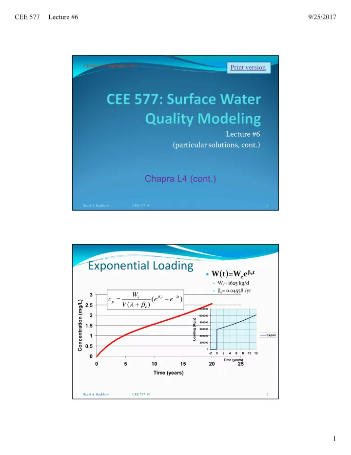
CEE 577 Lecture #6 9/25/2017 Updated: 25 September 2017 Print version Lecture #6 (particular solutions, cont.) Chapra L4 (cont.) David A. Reckhow CEE 577 #6 1 Exponential Loading  W(t)=W e e  e t  W e = 1625 kg/d   e = 0.04558 /yr 3 W      ( t t ) e c e e e Concentration (mg/L)    p ( ) V 2.5 e 1200000 2 1000000 Loading (Kg/y) 800000 1.5 600000 1 Expon 400000 200000 0.5 0 -2 0 2 4 6 8 10 12 0 Time (years) 0 5 10 15 20 25 Time (years) David A. Reckhow CEE 577 #6 2 1

CEE 577 Lecture #6 9/25/2017  W(t)=W ‐ bar+ W a sin(  t ‐  ) Sinusoidal Loading  W ‐ bar= 500,000 kg/yr  W a = 250,000 kg/yr T p   T p = 2  = 1 yr  phase shift,  = (0.25)2  =0.5  1000000 900000 800000 Loading (Kg/y) 700000 W a 600000 500000 400000 300000 W-bar 200000 100000 0 -1 -0.5 0 0.5 1 1.5 2 Time (years) David A. Reckhow CEE 577 #6 3 W-bar= 500,000 kg/yr W a = 250,000 kg/yr Sinusoidal Loading T p = 2  = 1 year phase shift ,  = 0.5     Response 1.2    ( ) arctan      phase shift Concentration (mg/L) 1 0.8 0.6 W W              ( 1 t ) sin ( ) a c e t p     2 2 0.4 V V W   0.2         sin ( ) exp( ) a t  2   2 V 0 0 5 10 15 20 25 1200000 1000000 Loading (Kg/y) Time (years) 800000 600000 Sinusoid 400000 Return 200000 0 -2 0 2 4 6 8 10 12 Time (years) David A. Reckhow CEE 577 #6 4 2

CEE 577 Lecture #6 9/25/2017 Q=2x10 5 m 3 /d A=1.1x10 8 m 2 V=1.75x10 9 3 Sinusoidal Loading k  0   0 042 . Increasing  k  0 0003 .   015 . k  0 001 .   0 42 . k  0 005 .   187 . David A. Reckhow CEE 577 #6 5 Example (similar to: 11.1 from Reckhow & Chapra)  Green Lake & Happy Valley  Hydraulic Parameters  Q=20x10 6 m 3 /yr, V=100x10 6 m 2 , A s =10x10 6 m 2 , H=10m  Decay: k=1.05/yr  Loading  local WWTP: 0.115x10 4 g/capita/yr, 20,000 people (long term, but at t=0, WW is pumped to regional plant)  new paper mill: 50x10 6 g/yr  new cattle feed lot: 150 animals, increasing by 100 cattle each year, 0.1x10 6 g/animal  New scenario: regional WWTP cannot accept new WW, town of Happy Valley is growing exponentially at 0.3/yr  New canning plant: annual cycle, avg=30x10 6 g/yr  max on Oct 1; min on Apr 1 (half of average) David A. Reckhow CEE 577 #6 6 3

CEE 577 Lecture #6 9/25/2017 Summation of Loading Summation 4 Concentration (mg/L) 3.5 Cattle Feed Lot 3 2.5 WWTP 2 1.5 Canning plant 1 0.5 Paper Mill 0 Decay of C o 0 5 10 15 20 25 Time (years) David A. Reckhow CEE 577 #6 7 WWTP: dirunal variations  Figures 1.6 a & b, from Thomann & Mueller David A. Reckhow CEE 577 #6 8 4

CEE 577 Lecture #6 9/25/2017 WWTP: weekly variations  Figure 1.6 c, from Thomann & Mueller David A. Reckhow CEE 577 #6 9 WWTP: Seasonal Variations  Figure 1.6 d, from Thomann & Mueller David A. Reckhow CEE 577 #6 10 5

CEE 577 Lecture #6 9/25/2017 Next: Cultural Eutrophication  Many correlated WQ problems  Floating mats of algae  Low DO  High P? David A. Reckhow CEE 577 #6 11  To next lecture David A. Reckhow CEE 577 #6 12 6