Experimental Quantum Physics The starting point Level 0.1: We want to - - PDF document

experimental quantum physics
SMART_READER_LITE
LIVE PREVIEW

Experimental Quantum Physics The starting point Level 0.1: We want to - - PDF document

Experimental Quantum Physics The starting point Level 0.1: We want to have fun with experimental quantum mechanics and gain as much control as possible over the processes Level 1.0: Do something useful with the systems: e.g


slide-1
SLIDE 1

Experimental Quantum Physics

The starting point

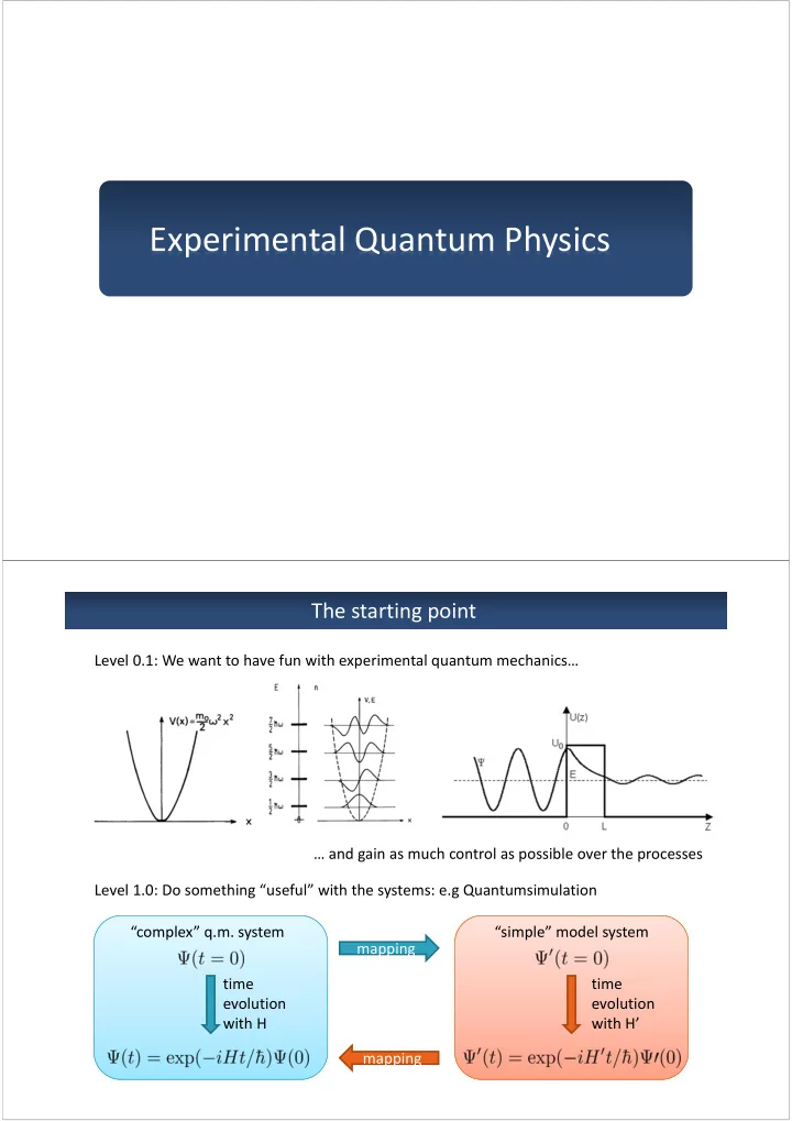
Level 0.1: We want to have fun with experimental quantum mechanics… … and gain as much control as possible over the processes Level 1.0: Do something “useful” with the systems: e.g Quantumsimulation “complex” q.m. system time evolution with H “simple” model system mapping time evolution with H’ mapping

slide-2
SLIDE 2

There are various ways to generate that, we will only consider neutral atoms

We need a quantum lab!

One of the main ingredients of the quantum laboratory

T>>Tc T~Tc T=0

d v dB

Bose Einstein Condensate

  • Macroscopic occupation of one quantum

mechanical level

  • Coherent matter wave :

matter wave interference

  • Interaction between atoms dominates

ground state as well as dynamical behavior

Some properties of BEC

  • Excellent control over all (most,…)

experimental parameters

Theoretical prediction 1924/5: A. Einstein and S. N. Bose First experimental realization 1995 BEC in dilute alkali gases: E. A. Cornell, W. Ketterle and C. E. Wieman

slide-3
SLIDE 3

Experimental realization of BEC

2D‐MOT 3D‐MOT Molasses

Magnetic trap Evaporation

n=104cm‐3 T=300K

n=1010cm‐3 T=10‐100µK n=1014cm‐3 T=100nK

Laser cooling

Experimental realization of BEC

n=104cm‐3 T=300K

n=1010cm‐3 T=10‐100µK n=1014cm‐3 T=100nK

Laser cooling

2D‐MOT 3D‐MOT Molasses

Magnetic trap Evaporation

slide-4
SLIDE 4

2D‐MOT 3D‐MOT Molasses

Magnetic trap Evaporation

Dipol trap n=104cm‐3 T=300K

n=1010cm‐3 T=10‐100µK

n=1014cm‐3 T=100nK n=1014cm‐3 T=100nK

Particle number from 1010 down to 106

Experimental realization of BEC

2D‐MOT 3D‐MOT Molasses Magnetic trap Evaporation

Dipole trap

n=104cm‐3 T=300K n=1010cm‐3 T=10‐100µK

n=1014cm‐3 T=100nK

Isotropic trap Elongated trap

Experimental realization of BEC

slide-5
SLIDE 5

2D‐MOT 3D‐MOT Molasses

Magnetic trap Evaporation

n=104cm‐3 T=300K

n=1010cm‐3 T=10‐100µK

n=1014cm‐3 T=100nK n=1014cm‐3 T=100nK

Particle number from 1010 down to 106

Experimental realization of BEC One, two,…more…

Degenerate Bose gas Exploiting the different quantum statistics Degenerate Fermi gas Various combinations:

  • Bose – Fermi mixtures
  • Fermionic Molecules
  • Mixtures of spin

components

  • Bosonic molecules
slide-6
SLIDE 6

Physics with Bose‐Einstein condensates

Bloch, Munich

Atom Laser

Ketterle, MIT

Collective excitations

Greiner, MPQ

Optical lattices Molecular BEC

Grimm, Innsbruck

Multi component BEC

Hamburg

Low‐dimensional systems

Paredes, MPQ

BEC

Ok, so we have a fancy quantum mechanical system with quite some control, but what to simulate with it?

Non‐exclusive choice of applications

Motivation and Applications

  • Almost arbitrary lattice geometries

can be realized using interfering laser beams

  • No lattice imperfections
  • No impurity atoms (only if desired)
  • Continuous tuning of lattice

parameters

  • Almost perfect model system

Benefits of OL

  • Solid state models
  • Quantum magnetism
  • Cold chemistry
  • Atomic clocks
  • Quantum information
  • Exotic super conductors
slide-7
SLIDE 7

Back to some basic atomic physics

Light

  • The two systems couple together via

electric dipole transitions Transition matrix element Coupling of the two systems leads to a shift of the energy levels The shift is proportional to ∆~ ∙

~

In words: The (potential) energy of the respective atomic level depends on the intensity distribution of the light field Atom

  • |

| | | |, ,

Atoms in an off‐resonant laser beam

Neutral Atom Time dependent electric field

+ →

Induced dipole moment Induced dipole moment interacts with the electric field Force onto the atom

slide-8
SLIDE 8

Periodic potentials

Simplest case: 1D lattice by retro reflecting a laser beam Optical dipole potential:

  • Potential is proportional to the

intensity distribution of the light field

  • Sign depends on wavelength of the

laser (usually “‐“)

Optical lattices: Light crystals

Laser Laser Optical lattice : laser interference Potential for polarizable atoms Lattice beam intensity (lattice depth) Tunnel rate Optical lattices:

  • No phonons (Lattice structure is rigid)
  • No localized impurities or defects
  • Highly controllable !
  • Kin. energy
  • Int. energy

Interactions Periodic potential Solid: ionic crystal Potential for electrons Band structure

16

slide-9
SLIDE 9

Ways to measure what‘s going on

Direct site resolved imaging Weiss, Greiner, Bloch and other labs Ott lab Imaging after release from lattice

Resonant Imaging Beam

CCD camera

Laser Laser

In‐situ momentum distribution is converted into real space due to free expansion

Tuneable lattice geometries

Most simple case: make the mutually orthogonal sets of beams independent V x, y, z ~

, cos , cos , cos

Greiner et al.

slide-10
SLIDE 10

Dimensionality and Geometry

Kagomé Honeycomb Triangular

Jo et al.,Phys. Rev. Lett. 108, 045305 (2012) Soltan‐Panahi et al., Nature Physics 7, 434 (2011) Tarruell et al., Nature 483, 302 (2012) Becker et al., New J. Phys. 12, 065025 (2010) Overview on novel geometries: Windpassinger & Sengstock

  • Rep. Prog. Phys. 76, 086401 (2013)

Toolbox of tunable lattice geometries

Double well lattices Variable geometries

e.g. J. Porto (NIST),

  • A. Hemmerich (Hamburg),
  • I. Bloch (MUC),
  • M. Weitz (Bonn)
  • D. Stamper‐Kurn (Berkeley)
  • T. Esslinger (ETH)
  • K. Sengstock

(Hamburg)

Windpassinger & Sengstock

  • Rep. Prog. Phys. 76, 086401 (2013)