Example: Grid World CS 188: Artificial Intelligence Markov Decision - PowerPoint PPT Presentation

Example: Grid World CS 188: Artificial Intelligence Markov Decision Processes II � A maze-like problem � The agent lives in a grid � Walls block the agent’s path � Noisy movement: actions do not always go as planned � 80% of the time, the action North takes the agent North � 10% of the time, North takes the agent West; 10% East � If there is a wall in the direction the agent would have been taken, the agent stays put � The agent receives rewards each time step � Small “living” reward each step (can be negative) � Big rewards come at the end (good or bad) � Goal: maximize sum of (discounted) rewards Instructors: Dan Klein and Pieter Abbeel --- University of California, Berkeley [These slides were created by Dan Klein and Pieter Abbeel for CS188 Intro to AI at UC Berkeley. 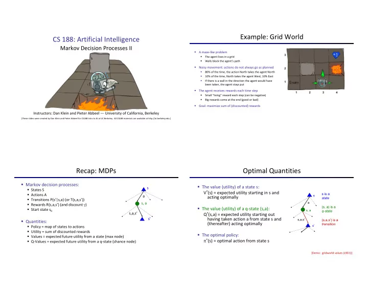All CS188 materials are available at http://ai.berkeley.edu.] Recap: MDPs Optimal Quantities � Markov decision processes: � The value (utility) of a state s: s � States S V * (s) = expected utility starting in s and s is a � Actions A s a acting optimally state � Transitions P(s’|s,a) (or T(s,a,s’)) a s, a � Rewards R(s,a,s’) (and discount γ ) (s, a) is a � The value (utility) of a q-state (s,a): � Start state s 0 s, a q-state s,a,s’ Q * (s,a) = expected utility starting out s’ having taken action a from state s and s,a,s’ (s,a,s’) is a � Quantities: (thereafter) acting optimally transition s’ � Policy = map of states to actions � Utility = sum of discounted rewards � The optimal policy: � Values = expected future utility from a state (max node) π * (s) = optimal action from state s � Q-Values = expected future utility from a q-state (chance node) [Demo: gridworld values (L9D1)]

Gridworld Values V* Gridworld: Q* The Bellman Equations The Bellman Equations � Definition of “optimal utility” via expectimax s recurrence gives a simple one-step lookahead a How to be optimal: relationship amongst optimal utility values s, a Step 1: Take correct first action s,a,s’ Step 2: Keep being optimal s’ � These are the Bellman equations, and they characterize optimal values in a way we’ll use over and over

Value Iteration Convergence* � Bellman equations characterize the optimal values: � How do we know the V k vectors are going to converge? V(s) � Case 1: If the tree has maximum depth M, then V M holds a the actual untruncated values s, a � Case 2: If the discount is less than 1 s,a,s’ � Sketch: For any state V k and V k+1 can be viewed as depth � Value iteration computes them: V(s’) k+1 expectimax results in nearly identical search trees � The difference is that on the bottom layer, V k+1 has actual rewards while V k has zeros � That last layer is at best all R MAX � It is at worst R MIN � But everything is discounted by γ k that far out � Value iteration is just a fixed point solution method � So V k and V k+1 are at most γ k max|R| different � … though the V k vectors are also interpretable as time-limited values � So as k increases, the values converge Policy Methods Policy Evaluation

Fixed Policies Utilities for a Fixed Policy Do what π says to do Do the optimal action � Another basic operation: compute the utility of a state s s under a fixed (generally non-optimal) policy s s π (s) π (s) a � Define the utility of a state s, under a fixed policy π : s, π (s) s, π (s) s, a V π (s) = expected total discounted rewards starting in s and following π s, π (s),s’ s, π (s),s’ s,a,s’ � Recursive relation (one-step look-ahead / Bellman equation): s’ s’ s’ � Expectimax trees max over all actions to compute the optimal values � If we fixed some policy π (s), then the tree would be simpler – only one action per state � … though the tree’s value would depend on which policy we fixed Example: Policy Evaluation Example: Policy Evaluation Always Go Right Always Go Forward Always Go Right Always Go Forward

Policy Evaluation Policy Extraction � How do we calculate the V’s for a fixed policy π ? s π (s) � Idea 1: Turn recursive Bellman equations into updates (like value iteration) s, π (s) s, π (s),s’ s’ � Efficiency: O(S 2 ) per iteration � Idea 2: Without the maxes, the Bellman equations are just a linear system � Solve with Matlab (or your favorite linear system solver) Computing Actions from Values Computing Actions from Q-Values � Let’s imagine we have the optimal values V*(s) � Let’s imagine we have the optimal q-values: � How should we act? � How should we act? � It’s not obvious! � Completely trivial to decide! � We need to do a mini-expectimax (one step) � This is called policy extraction, since it gets the policy implied by the values � Important lesson: actions are easier to select from q-values than values!

Policy Iteration Problems with Value Iteration � Value iteration repeats the Bellman updates: s a s, a s,a,s’ � Problem 1: It’s slow – O(S 2 A) per iteration s’ � Problem 2: The “max” at each state rarely changes � Problem 3: The policy often converges long before the values [Demo: value iteration (L9D2)] k=0 k=1 Noise = 0.2 Noise = 0.2 Discount = 0.9 Discount = 0.9 Living reward = 0 Living reward = 0

k=2 k=3 Noise = 0.2 Noise = 0.2 Discount = 0.9 Discount = 0.9 Living reward = 0 Living reward = 0 k=4 k=5 Noise = 0.2 Noise = 0.2 Discount = 0.9 Discount = 0.9 Living reward = 0 Living reward = 0

k=6 k=7 Noise = 0.2 Noise = 0.2 Discount = 0.9 Discount = 0.9 Living reward = 0 Living reward = 0 k=8 k=9 Noise = 0.2 Noise = 0.2 Discount = 0.9 Discount = 0.9 Living reward = 0 Living reward = 0

k=10 k=11 Noise = 0.2 Noise = 0.2 Discount = 0.9 Discount = 0.9 Living reward = 0 Living reward = 0 k=12 k=100 Noise = 0.2 Noise = 0.2 Discount = 0.9 Discount = 0.9 Living reward = 0 Living reward = 0

Policy Iteration Policy Iteration � Alternative approach for optimal values: � Evaluation: For fixed current policy π , find values with policy evaluation: � Step 1: Policy evaluation: calculate utilities for some fixed policy (not optimal � Iterate until values converge: utilities!) until convergence � Step 2: Policy improvement: update policy using one-step look-ahead with resulting converged (but not optimal!) utilities as future values � Repeat steps until policy converges � Improvement: For fixed values, get a better policy using policy extraction � One-step look-ahead: � This is policy iteration � It’s still optimal! � Can converge (much) faster under some conditions Comparison Summary: MDP Algorithms � So you want to…. � Both value iteration and policy iteration compute the same thing (all optimal values) � Compute optimal values: use value iteration or policy iteration � In value iteration: � Compute values for a particular policy: use policy evaluation � Every iteration updates both the values and (implicitly) the policy � Turn your values into a policy: use policy extraction (one-step lookahead) � We don’t track the policy, but taking the max over actions implicitly recomputes it � In policy iteration: � These all look the same! � We do several passes that update utilities with fixed policy (each pass is fast because we � They basically are – they are all variations of Bellman updates consider only one action, not all of them) � They all use one-step lookahead expectimax fragments � After the policy is evaluated, a new policy is chosen (slow like a value iteration pass) � They differ only in whether we plug in a fixed policy or max over actions � The new policy will be better (or we’re done) � Both are dynamic programs for solving MDPs

Double Bandits Double-Bandit MDP � Actions: Blue, Red No discount � States: Win, Lose 100 time steps 0.25 $0 Both states have the same value 0.75 $2 0.25 W L $0 $1 $1 0.75 $2 1.0 1.0 Offline Planning Let’s Play! � Solving MDPs is offline planning No discount � You determine all quantities through computation 100 time steps � You need to know the details of the MDP Both states have the same value � You do not actually play the game! 0.25 $0 Value 0.75 0.25 W $2 L Play Red 150 $2 $2 $0 $2 $2 $0 $1 $1 0.75 $2 $2 $2 $0 $0 $0 Play Blue 100 1.0 1.0

Online Planning Let’s Play! � Rules changed! Red’s win chance is different. ?? $0 ?? $2 ?? W L $0 $1 $1 ?? $2 $0 $0 $0 $2 $0 1.0 1.0 $2 $0 $0 $0 $0 What Just Happened? Next Time: Reinforcement Learning! � That wasn’t planning, it was learning! � Specifically, reinforcement learning � There was an MDP, but you couldn’t solve it with just computation � You needed to actually act to figure it out � Important ideas in reinforcement learning that came up � Exploration: you have to try unknown actions to get information � Exploitation: eventually, you have to use what you know � Regret: even if you learn intelligently, you make mistakes � Sampling: because of chance, you have to try things repeatedly � Difficulty: learning can be much harder than solving a known MDP