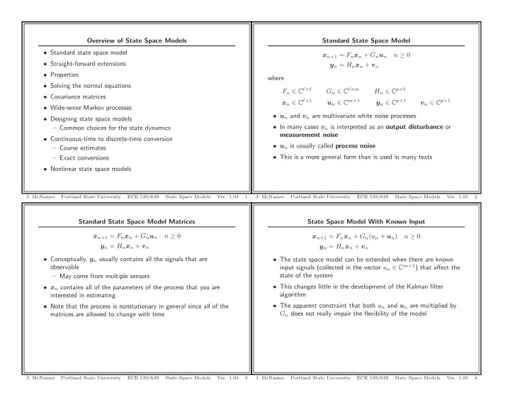
overview of state space models standard state space model
play

Overview of State Space Models Standard State Space Model Standard - PowerPoint PPT Presentation

Overview of State Space Models Standard State Space Model Standard state space model x n +1 = F n x n + G n u n n 0 Straight-forward extensions y n = H n x n + v n Properties where Solving the normal equations F n C


  1. Overview of State Space Models Standard State Space Model • Standard state space model x n +1 = F n x n + G n u n n ≥ 0 • Straight-forward extensions y n = H n x n + v n • Properties where • Solving the normal equations F n ∈ C ℓ × ℓ G n ∈ C ℓ × m H n ∈ C p × ℓ • Covariance matrices x n ∈ C ℓ × 1 u n ∈ C m × 1 y n ∈ C p × 1 v n ∈ C p × 1 • Wide-sense Markov processes • u n and v n are multivariate white noise processes • Designing state space models • In many cases v n is interpreted as an output disturbance or – Common choices for the state dynamics measurement noise • Continuous-time to discrete-time conversion • u n is usually called process noise – Coarse estimates • This is a more general form than is used in many texts – Exact conversions • Nonlinear state space models J. McNames Portland State University ECE 539/639 State Space Models Ver. 1.03 1 J. McNames Portland State University ECE 539/639 State Space Models Ver. 1.03 2 Standard State Space Model Matrices State Space Model With Known Input x n +1 = F n x n + G n u n n ≥ 0 x n +1 = F n x n + G n ( u n + u n ) n ≥ 0 y n = H n x n + v n y n = H n x n + v n • Conceptually, y n usually contains all the signals that are • The state space model can be extended when there are known input signals (collected in the vector u n ∈ C m × 1 ) that affect the observable state of the system – May come from multiple sensors • This changes little in the development of the Kalman filter • x n contains all of the parameters of the process that you are algorithm interested in estimating • The apparent constraint that both u n and u n are multiplied by • Note that the process is nonstationary in general since all of the G n does not really impair the flexibility of the model matrices are allowed to change with time J. McNames Portland State University ECE 539/639 State Space Models Ver. 1.03 3 J. McNames Portland State University ECE 539/639 State Space Models Ver. 1.03 4

  2. State Space Model With Known Input Continued State Space Model With Known Input Continued x n +1 = F n x n + G n u n x n +1 = F n x n + G n ( u n + u n ) n ≥ 0 y n = H n x n + v n y n = H n x n + v n • An additional known input signal could be added to the output • We can specify the covariance matrix of u n to be anything we like equation in a similar fashion such that the additive noise term has whatever covariance matrix we like y n = H n x n + w n + v n • Suppose we wish for the scaled state noise G n u n to have a • This is most easily handled by defining a different observed signal covariance matrix T n as Q n � G − 1 n T n G −∗ n z n � y n − w n � u n , u n � = Q n z n = H n x n + v n � G n u n , G n u n � = G n Q n G ∗ n = T n • Thus, it easily reduces to the form of our standard state space model output equation J. McNames Portland State University ECE 539/639 State Space Models Ver. 1.03 5 J. McNames Portland State University ECE 539/639 State Space Models Ver. 1.03 6 Covariance Matrices Covariance Matrices ⎡ ⎤ x 0 x n +1 = F n x n + G n u n �⎡ ⎤ ⎡ ⎤ x 0 Π 0 0 0 0 � x n +1 = F n x n + G n u n u k y n = H n x n + v n ⎦ , ⎢ ⎥ u n = 0 Q n δ nk S n δ nk 0 ⎣ ⎢ ⎥ ⎣ ⎦ y n = H n x n + v n v k ⎣ ⎦ S ∗ 0 n δ nk R n δ nk 0 v n ⎡ ⎤ x 0 1 �⎡ ⎤ ⎡ ⎤ x 0 Π 0 0 0 0 � u k ⎦ , ⎢ ⎥ u n = 0 Q n δ nk S n δ nk 0 • The matrices Π 0 , Q n , R n , and S n are assumed to be known ⎣ ⎢ ⎥ ⎣ ⎦ v k ⎣ ⎦ S ∗ 0 n δ nk R n δ nk 0 v n 1 • By definition, the matrices Q n and R n must be Hermitian and non-negative definite • The random variable x 0 and the two white noise processes drive • The matrix S n doesn’t have to be Hermitian, but it must be such the state space model that the joint covariance matrix is non-negative definite – This means that � u n , u k � = 0 for n � = k – Does not mean Q n or R n are diagonal matrices � � Q S ≥ 0 S ∗ R • The model is causal in that x n and y n are completely determined by x 0 and past and present values of v n and u n • This characterization ensures the process is wide-sense Markov (to • Clever use of the inner product notation has been used here to be discussed later) indicate these RVs have zero mean J. McNames Portland State University ECE 539/639 State Space Models Ver. 1.03 7 J. McNames Portland State University ECE 539/639 State Space Models Ver. 1.03 8

  3. Correlation of Process and Measurement Noise Orthogonality Properties ⎡ ⎤ You should be able to show that the following properties are true: x 0 �⎡ ⎤ ⎡ ⎤ x 0 Π 0 0 0 0 � x n +1 = F n x n + G n u n u k ⎦ , ⎢ ⎥ = 0 Q n δ nk S n δ nk 0 u n � u n , x k � = 0 � v n , x k � = 0 for n ≥ k ⎣ ⎢ ⎥ ⎣ ⎦ y n = H n x n + v n v k S ∗ ⎣ ⎦ v n 0 n δ nk R n δ nk 0 � u n , y k � = 0 � v n , y k � = 0 for n > k 1 � u n , y k � = S n � v n , y k � = R n for n = k • It is common to assume the process and measurement noise processes are completely uncorrelated, S n = 0 for all n � u n , x 0 � = 0 iff � u n , x n � = 0 for n ≥ 0 • Due to domain knowledge that they have different origins • The key idea is to leverage the orthogonality of the initial state • When feedback is used and the output modifies the state and the noise covariance matrices equation, the noises may become correlated, S n � = 0 for some n • There are many forms, but the most useful is to assume that they are correlated only at the same time instant J. McNames Portland State University ECE 539/639 State Space Models Ver. 1.03 9 J. McNames Portland State University ECE 539/639 State Space Models Ver. 1.03 10 Example 1: Orthogonality Properties Relationship to R y x n +1 = F n x n + G n u n x n | n = � x n , y �� y � − 2 y y � col { y 0 , . . . , y n } ˆ y n = H n x n + v n • We know that the optimal causal estimator of x n is given by the Prove some of the orthogonality properties on the previous slide. normal equations • Requires knowledge of two terms • The first is easy to solve for � x n , y � = � x n , H n x n + v n � = � x n , x n � H ∗ n • In order to solve the normal equations, we need to know how R y = � y � 2 is related to all of the state space model parameters and covariance matrices • However, we need to solve for � x n , x k � in order to obtain expressions for both � x n , y � and R y J. McNames Portland State University ECE 539/639 State Space Models Ver. 1.03 11 J. McNames Portland State University ECE 539/639 State Space Models Ver. 1.03 12

  4. Solving for the State Covariance Matrix Solving for the State Covariance Matrix Continued Given the state space model, Now let us define the state transition matrix � F n − 1 F n − 2 . . . F k n > k x n +1 = F n x n + G n u n Φ( n, k ) � I n = k y n = H n x n + v n Then we can easily show that Π n +1 � � x n , x n � x n = Φ( n, k ) x k + A col { u k , u k +1 , . . . , u n − 1 } , n ≥ k = � F n x n + G n u n , F n x n + G n u n � for some matrix A . In other words, x n consists of Φ( n, k ) x k plus = F n � x n , x n � F ∗ n + G n � u n , u n � G ∗ some linear combination of { u k , u k +1 , . . . , u n − 1 } , which is n = F n Π n F ∗ n + G n Q n G ∗ uncorrelated with x k . Thus n � x n , x k � = � Φ( n, k ) x k + A col { u k , u k +1 , . . . , u n − 1 } , x k � = Φ( n, k ) � x k , x k � + 0 = Φ( n, k )Π k for n ≥ k J. McNames Portland State University ECE 539/639 State Space Models Ver. 1.03 13 J. McNames Portland State University ECE 539/639 State Space Models Ver. 1.03 14 Solving for the State Covariance Matrix Continued Solving for the Output Covariance Matrix R y Given the state space model, � x n , x k � = Φ( n, k )Π k for n ≥ k x n +1 = F n x n + G n u n For since � x , y � = � y , x � ∗ for any random vectors x and y , it follows y n = H n x n + v n immediately that The output covariance matrix is given by � x n , x k � = � x k , x n � ∗ = (Φ( k, n )Π n ) ∗ � y n , y k � = � H n x n + v n , H k x k + v k � = H n � x n , x k � H ∗ k + H n � x n , v k � + � v n , x k � H ∗ = Π n Φ ∗ ( k, n ) for n ≤ k k + � v n , v k � The cross-terms � x n , v k � and � v n , x k � don’t necessarily cancel in this These results can be summarized as case sense u n and v n are correlated. ⎧ Φ( n, k )Π k n ≥ k However they do if n = k since then x n is only a function of past ⎪ ⎨ values of u n � x n , x k � = Π n n = k ⎪ Π n Φ ∗ ( k, n ) n ≤ k ⎩ If � v n , x k � = 0 � x n , v k � = 0 � y n , y n � = H n Π n H ∗ then n + R n J. McNames Portland State University ECE 539/639 State Space Models Ver. 1.03 15 J. McNames Portland State University ECE 539/639 State Space Models Ver. 1.03 16

Download Presentation
Download Policy: The content available on the website is offered to you 'AS IS' for your personal information and use only. It cannot be commercialized, licensed, or distributed on other websites without prior consent from the author. To download a presentation, simply click this link. If you encounter any difficulties during the download process, it's possible that the publisher has removed the file from their server.

Recommend


More recommend