Probabilistic Graphical Models 10-708 Factor Analysis and State - PDF document

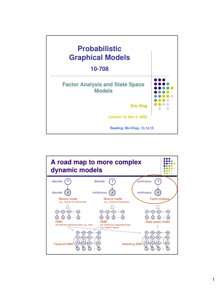
Probabilistic Graphical Models 10-708 Factor Analysis and State Space Factor Analysis and State Space Models Models Eric Xing Eric Xing Lecture 15, Nov 2, 2005 Reading: MJ-Chap. 13,14,15 A road map to more complex dynamic models Y Y Y discrete discrete continuous discrete continuous continuous A X X A X A Mixture model Mixture model Factor analysis e.g., mixture of multinomials e.g., mixture of Gaussians y 1 y 1 y 2 y 2 y 3 y 3 y N y N y 1 y 1 y 2 y 2 y 3 y 3 y N y N y 1 y 1 y 2 y 2 y 3 y 3 y N y N ... ... ... ... ... ... x 1 A x 1 A A A x 2 x 2 A x 3 A x 3 x N x N A A x 1 A x 1 A x 2 x 2 A A x 3 A x 3 A x N x N A A x 1 A x 1 A x 2 x 2 A A x 3 x 3 A A x N x N A A ... ... ... ... ... ... HMM HMM State space model (for discrete sequential data, e.g., text) (for continuous sequential data, e.g., speech signal) S 1 S 1 S 2 S 2 S 3 S 3 S N S N S 1 S 1 S 2 S 2 S 3 S 3 S N S N ... ... ... ... y 11 y 11 y 12 y 12 y 13 y 13 y 1N y 1N y 11 y 11 y 12 y 12 y 13 y 13 y 1N y 1N ... ... ... ... ... ... ... ... ... ... ... ... ... ... ... ... ... ... ... ... y k1 y k1 y k2 y k2 y k3 y k3 y kN y kN y k1 y k1 y k2 y k2 y k3 y k3 y kN y kN Factorial HMM ... ... Switching SSM ... ... A x 1 A x 1 A x 2 x 2 A A A x 3 x 3 x N x N A A x 1 A x 1 A x 2 A x 2 A x 3 A A x 3 x N A A x N ... ... ... ... 1

Review: A primer to multivariate Gaussian � Multivariate Gaussian density: 1 { } p T − 1 µ Σ = 1 µ Σ µ ( | , ) exp - ( - ) ( - ) x x x 2 1 2 2 n 2 π Σ / / ( ) � A joint Gaussian: ⎡ ⎤ ⎡ ⎤ ⎡ µ ⎤ ⎡ Σ Σ ⎤ x x p 1 1 1 11 12 µ Σ = N ( ⎢ ⎥ | , ) ( ⎢ ⎥ ⎢ ⎥ , ⎢ ⎥ ) µ Σ Σ ⎣ x ⎦ ⎣ x ⎦ ⎣ ⎦ ⎣ ⎦ 2 2 2 21 22 � How to write down p ( x 1 ), p ( x 1 | x 2 ) or p ( x 2 | x 1 ) using the block elements in µ and Σ ? � Formulas to remember: p p m m = N = N ( ) ( | , ) ( ) ( | , ) x x x m V x x m V 1 2 1 1 2 1 2 2 2 2 2 | | m 1 = µ = µ + Σ Σ − − µ ( ) m m x 2 2 1 2 1 12 22 2 2 | m = Σ 1 = Σ − Σ Σ − Σ V V 2 22 1 2 11 12 22 21 | Review: The matrix inverse lemma ⎡ ⎤ E F = � Consider a block-partitioned matrix: M ⎢ ⎥ ⎣ G H ⎦ � First we diagonalize M ⎡ ⎤ ⎡ ⎤ ⎡ ⎤ ⎡ ⎤ H - 1 H - 1 - F E F 0 E - F G 0 I I = ⎢ ⎥ ⎢ ⎥ ⎢ ⎥ ⎢ ⎥ H 1 - ⎣ ⎦ ⎣ G H ⎦ ⎣ G ⎦ ⎣ H ⎦ 0 - 0 I I = M H H - 1 Schur complement: E G � - F / = ⇒ = W W � Then we inverse, using this formula: - 1 - 1 X Y Y X Z Z − 1 ( ) 1 ⎡ ⎤ ⎡ ⎤ ⎡ − ⎤ ⎡ ⎤ M H - 1 E F 0 H - F 0 − 1 I = = / I ⎢ ⎥ ⎢ ⎥ M ⎢ ⎥ ⎢ ⎥ − 1 ⎣ H ⎦ ⎣ - 1 ⎦ G H G ⎣ H ⎦ ⎣ ⎦ - 0 0 I I ( ) ( ) ( ) ( ) ⎡ − 1 − 1 ⎤ ⎡ − 1 − 1 ⎤ − 1 + − 1 − 1 M M M M H H H - 1 G - 1 - F E E F E E - E F E = / / = / / ⎢ ⎥ ⎢ ⎥ ( ) ( ) ( ) ( ) 1 − 1 1 1 − 1 − 1 − 1 − − + − M M - M - M ⎣ H G H H H G H H 1 ⎦ ⎣ G 1 ⎦ - F - E E E / / / / � Matrix inverse lemma ( ) ( ) − 1 − 1 1 1 = − + − H - 1 H - 1 - 1 E G E E G E F G E - F F - 2

Review: Some matrix algebra [ ] ∑ def a � Trace and derivatives = tr A ii i Cyclical permutations � [ ] [ ] [ ] = = tr tr tr ABC CAB BCA Derivatives � ∂ tr [ ] = T BA B ∂ A ∂ [ ] ∂ [ ] = = T T T tr tr x Ax xx A xx ∂ ∂ A A � Determinants and derivatives ∂ log = -T A A ∂ A Factor analysis � An unsupervised linear regression model p 0 = N ( ) ( ; , ) x x I X p = µ + Λ Ψ N ( x y ) ( y ; x , ) where Λ is called a factor loading matrix, and Ψ is diagonal. A Y � Geometric interpretation To generate data, first generate a point within the manifold then add � noise. Coordinates of point are components of latent variable. 3

Marginal data distribution � A marginal Gaussian (e.g., p ( x )) times a conditional Gaussian (e.g., p ( y | x )) is a joint Gaussian � Any marginal (e.g., p ( y ) of a joint Gaussian (e.g., p ( x , y )) is also a Gaussian Since the marginal is Gaussian, we can determine it by just computing � its mean and variance. (Assume noise uncorrelated with data.) [ ] [ ] 0 = µ + Λ + N Ψ E Y E X W w here W ~ ( , ) [ ] [ ] = µ + Λ + E X E W 0 0 = µ + + = µ [ ] [ ] ( )( ) = − µ − µ T Var Y E Y Y [ ] ( )( ) = µ + Λ + − µ µ + Λ + − µ T E X W X W [ ] ( )( ) = Λ + Λ + T X W X W E [ ] [ ] = Λ Λ + T T T E XX E WW = ΛΛ + Ψ T FA = Constrained-Covariance Gaussian � Marginal density for factor analysis ( y is p -dim, x is k -dim): p θ = N µ ΛΛ + Ψ T ( | ) ( ; , ) y y � So the effective covariance is the low-rank outer product of two long skinny matrices plus a diagonal matrix: � In other words, factor analysis is just a constrained Gaussian model. (If were not diagonal then we could model any Gaussian and it would be pointless.) 4

FA joint distribution � Model p 0 = N ( ) ( ; , ) x x I p = N µ + Λ Ψ ( ) ( ; , ) y x y x � Covariance between x and y [ ] [ ] [ ] ( )( ) ( ) 0 = − − µ T = µ + Λ + − µ T Cov X, Y E X Y E x X W [ ] = Λ + T T T E XX xW = Λ T � Hence the joint distribution of x and y : 0 ⎡ ⎤ ⎡ ⎤ ⎡ ⎤ ⎡ ⎤ Λ x x T I p = N ( ) ( , ⎢ ⎥ ) ⎢ ⎥ ⎢ ⎥ ⎢ ⎥ µ Λ ΛΛ + Ψ ⎣ ⎦ ⎣ ⎦ ⎣ ⎦ T y y ⎣ ⎦ � Assume noise is uncorrelated with data or latent variables. Inference in Factor Analysis � Apply the Gaussian conditioning formulas to the joint distribution we derived above, where Σ = I 11 Σ = Σ = Λ T T 12 12 ( ) Σ = ΛΛ + Ψ T 22 we can now derive the posterior of the latent variable x given p = N observation y , , where ( ) ( | , ) x y x m V 1 2 1 2 | | = µ + Σ Σ − 1 − µ = Σ − Σ Σ − 1 Σ ( ) m y V 1 2 1 12 22 2 1 2 11 12 22 21 | | ( ) ( ) Λ − 1 − 1 = Λ ΛΛ + Ψ − µ = − Λ ΛΛ + Ψ T T T T ( ) y I ( ) ( ) 1 1 − − Applying the matrix inversion lemma = − 1 + − 1 H - 1 H G - 1 G - 1 E - F G E E F - E F E ( ) ⇒ ⇒ − Λ 1 − 1 − y 1 = + Λ Ψ = Λ Ψ − µ T T m V ( ) V I 1 2 1 2 1 2 | | | Here we only need to invert a matrix of size | x | × | x |, instead of | y | × | y |. � 5

Geometric interpretation: inference is linear projection � The posterior is: p = N ( x y ) ( x ; m , V ) 1 2 1 2 | | ( ) − Λ 1 − 1 − y 1 = + Λ Ψ = Λ Ψ − µ T T ( ) V I m V 1 2 1 2 1 2 | | | � Posterior covariance does not depend on observed data y ! � Computing the posterior mean is just a linear operation: EM for Factor Analysis � Incomplete data log likelihood function (marginal density of y) N 1 ( ) 1 ∑ T − D y y l θ = − ΛΛ + Ψ − − µ ΛΛ + Ψ − µ T T ( , ) log ( ) ( ) 2 2 n n n [ ] N 1 ( ) 1 ∑ − y µ y µ T = − ΛΛ + Ψ − ΛΛ + Ψ = − − T T log tr , where ( ) ( ) S S n n 2 2 n ∑ µ ML = 1 y � Estimating m is trivial: ˆ N n n Parameters Λ and Ψ are coupled nonlinearly in log-likelihood � � Complete log likelihood ∑ ∑ D p x y p x p y x l θ = = + ( , ) log ( , ) log ( ) log ( | ) n n n n n c n n N 1 N 1 ∑ ∑ T x T x y x 1 y x = − − − Ψ − − Λ Ψ − − Λ log log ( ) ( ) I 2 2 n n 2 2 n n n n n n N 1 N [ ] 1 ∑ ∑ = − Ψ − x T x − Ψ − 1 = y − Λ x y − Λ x T log tr , where ( ) ( ) S S n n n n n n 2 2 2 N n n 6