
SLIDE 1
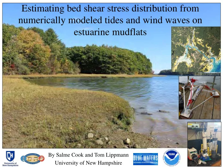
Estimating bed shear stress distribution from numerically modeled tides and wind waves on estuarine mudflats
By Salme Cook and Tom Lippmann University of New Hampshire
Estimating bed shear stress distribution from numerically modeled - - PowerPoint PPT Presentation
Estimating bed shear stress distribution from numerically modeled tides and wind waves on estuarine mudflats By Salme Cook and Tom Lippmann University of New Hampshire Estuaries Ocean River Mixing rain tides atmospheric seasonal Things
By Salme Cook and Tom Lippmann University of New Hampshire
Things that mix Salt Temperature Sediment Nutrients Pollutants
Mixing Processes Advection and Diffusion Turbulence tides atmospheric waves
rain seasonal
22 of the 32 largest cities in the world are located on estuaries 14% of coastal communities in the United States produce 45% of the nations GDP 76% of trade involves some form of marine transportation Coastal recreation brings in $8-12 Billion dollars to the United States every year
“buffer zone” that removes nutrients, sediment, and pollutants Nitrogen/Phosphorus Cycling Habitats ~ “Nursery of the sea” Shore stabilization/Flood regulation High primary productivity Carbon Sequestration
22 of the 32 largest cities in the world are located on estuaries 14% of coastal communities in the United States produce 45% of the nations GDP 76% of trade involves some form of marine transportation Coastal recreation brings in $8-12 Billion dollars to the United States every year
Habitats ~ “Nursery of the sea” “buffer zone” that removes nutrients, sediment, and pollutants Shore stabilization/Flood regulation Carbon Sequestration Nitrogen/Phosphorus Cycling High primary productivity
Wastewater Treatment Runoff : Fertilizer and Animal Waste
Industrial
Transportation Storm water Outfall
Applied Shear stress Sediment Resuspension Nutrient/Pollutant Release
Pore water Sediment
Based on sediment characteristics Hydrodynamics
Challenge: Cannot measure shear stress directly !
Z U(Z)
>50% mud fraction 0.35 N/m2 for nutrient release Percuoco (2013)
Distance above bed (Z)
Modified from Nielsen (1992)
Velocity (Z) Distance above bed (Z) Velocity (Z)
Quadratic Drag Logarithmic “law of the wall”
Function of the tidal current and a drag coefficient Function of the wave friction factor and wave
EPA - National Estuary Program (NEP) Tidally dominant (1-2 m/s currents; 2-4 m tide range) Low river input (<2% of tidal prism) Tidal Channels with fringing mudflats
Shchepetkin and McWilliams (2005), Shchepetkin et al., (2009a), Shchepetkin et al (2009b), and Haidvogel et al.,(2008)
Warner, J.C. et al (2009b) Warner, J.C. et al (2010)
Horizontal: 30 meter (and 10 meter) Vertical: 8 vertical sigma layers Grid Development
survey (CCOM - Paul Johnson)
FEMA, USGS) Gridding routines in Matlab to create a netcdf formatted file
Visualization using ParaView
Visualization using ParaView 5 km x 5 km
30 meter grid Model Configuration DT 1-1.5 s Horizontal Resolution 734 x 834 (22 km x 25 km) Vertical resolution 8 sigma layers Run Length 30 days zo 0.015 m, 0.020 m, 0.025 m, 0.030m Other: Wetting and Drying algorithm, Forcing ramped up over 1 day
Observations Subtidal Observations Tidal Predictions
30 meter grid Model Configuration DT 1-1.5 s Horizontal Resolution 734 x 834 (22 km x 25 km) Vertical resolution 8 sigma layers Run Length 30 days zo 0.015 m, 0.020 m, 0.025 m, 0.030m Other: Wetting and Drying algorithm, Forcing ramped up over 1 day
Observations Subtidal Observations Tidal Predictions Not that important Validated model Submitted to Ocean Modeling, May 2018
Classic Logarithmic “Law of the Wall” Formulation
u v zob
Lowest Water Cell High Tide Low Tide
Classic Logarithmic “Law of the Wall” Formulation
High Tide 2.8 m Low Tide 0.8 m
A B C
Kara Koetje, Diane Foster, Tom Lippmann
Tidal Signal (m) East-West & North-South Velocities (m/s) Velocity Magnitude (m/s)
Ebb Flood Flood Shear Stress Estimate: 0.41 N/m2 Ebb Shear Stress Estimate: 0.23 N/m2
Note: these observational estimates are preliminary
Flood Tide ~ 0.41 Ebb Tide ~ 0.23 Field Estimates Nutrient Release ~ 0.35 Lab Estimates
Nutrient Estimate: Step 1: Area with > 50% mud fraction Step 2: Area with shear stress > 0.35 N/m2 Step 3: Calculate Nutrient Load
0.35 N/m2 Bay Wide Estimate
Dissolved Inorganic Nitrogen (DIN) Phosphorus (P) (kg/month) (kg/month) River A (Fall, Sept-Nov) 1,200 70 (Winter, Dec-Feb) 3,700 92 (Spring, Mar-May) 17,000 720 (Summer, June-Aug) 1,300 120 Sediments (modeled) 2880 1020* (kg/event) (kg/event) Event (Storm-Irene) B 220 80* One Tidal Cycle (Average) 96 34* Neap Tide (Minimum) 13 5* Spring Tide (Maximum) 123 44*
A Oczkowski (2002) B Wengrove (2014)
* Based on results from Percuoco (2013). Uptake not considered for Phosphorus.
– (Cook et.al., Submitted May 2018/In Review - Ocean Modeling )
– Need more observation-based estimates of shear stress on mudflats across the bay (~1-2 masters students)
10 meter grid can only run on Blue Waters….
What about waves? Eel grass?
Tidal Boundary Wave Boundary
Z
U(Z)
Sediment Transport
resolution and zo
Capacitance Wave Gauge Spotter Buoy
UNH Wave Tank Great Bay, NH
Jim Irish Jamie Pringle (UNH) Chris Sherwood (USGS) Karl Kammerer (NOAA) Kara Koetje Diane Foster Mark Van Moer Jaehyuk Quak and many others…
Computations were performed on Trillian, a Cray XE6m-200 supercomputer at UNH supported by the NSF MRI program under grant PHY-1229408. (Jim Raeder) This research is part of the Blue Waters sustained-petascale computing project, which is supported by the National Science Foundation (awards OCI-0725070 and ACI-1238993) and the state of Illinois. Blue Waters is a joint effort of the University of Illinois at Urbana- Champaign and its National Center for Supercomputing Applications.
Los Angeles, USA Buenos Aires, Argentina NYC, USA Guangzhou, China Hong Kong Karachi, Pakistan Beijing, China Lagos, Nigeria Delhi, India Shanghai, China London, UK Seattle, USA Bangkok, Thailand Adelaide, AUS
CONCLUSIONS SHEAR STRESS MODEL GREAT BAY ESTUARY BACKGROUND MOTIVATION INTRODUCTION
CONCLUSIONS SHEAR STRESS MODEL GREAT BAY ESTUARY BACKGROUND MOTIVATION INTRODUCTION
National Estuary Program (NEP)
“Estuaries of National Significance”
Seattle,WA Portland, OR San Francisco, CA Los Angeles, CA Boston, MA New York City, NY Philadelphia, PA Washington DC New Orleans, LA Houston, TX
Vertical Structure of the Currents Observational Station Location (2015 field study)
Bottom (6.5 m)
North-South Direction
Surface Bottom (6.5 m)