Enhancing Voxel Carving by Capture Volume Calculations - - PowerPoint PPT Presentation

enhancing voxel carving by capture volume calculations
SMART_READER_LITE
LIVE PREVIEW

Enhancing Voxel Carving by Capture Volume Calculations - - PowerPoint PPT Presentation

Group on Human Motion Analysis Enhancing Voxel Carving by Capture Volume Calculations International Conference on Image Processing 2010 Tobias Feldmann, Karsten Brand, Annika W orner | February 23, 2011 G ROUP ON H UMAN M OTION A NALYSIS (G O


slide-1
SLIDE 1

GROUP ON HUMAN MOTION ANALYSIS (GO HU.MAN)
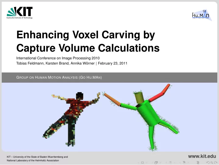
Group on Human Motion Analysis

Enhancing Voxel Carving by Capture Volume Calculations

International Conference on Image Processing 2010 Tobias Feldmann, Karsten Brand, Annika W¨

  • rner | February 23, 2011

KIT – University of the State of Baden-Wuerttemberg and National Laboratory of the Helmholtz Association

www.kit.edu

slide-2
SLIDE 2

Outline

1

Introduction

2

Basics Clipping Polygons With Half Spaces

3

Contribution Polyhedron, View Frustum and Adjacency Matrix Polyhedron clipping Problems in the real world Volume calculations

4

Evaluation

5

Conclusion

Introduction Basics Contribution Evaluation Conclusion Tobias Feldmann, Karsten Brand, Annika W¨

  • rner – Capture Volume Calculations

February 23, 2011 2/27

slide-3
SLIDE 3

Introduction

Dense volumetric reconstruction of gymnasts in sports. Multi camera based voxel carving approach.

Introduction Basics Contribution Evaluation Conclusion Tobias Feldmann, Karsten Brand, Annika W¨

  • rner – Capture Volume Calculations

February 23, 2011 3/27

slide-4
SLIDE 4

Problem Statement

During voxel based 3d reconstruction one question directly arises: Question: Which size for the reconstruction area?

Introduction Basics Contribution Evaluation Conclusion Tobias Feldmann, Karsten Brand, Annika W¨

  • rner – Capture Volume Calculations

February 23, 2011 4/27

slide-5
SLIDE 5

Problem Statement

During voxel based 3d reconstruction one question directly arises: Question: Which size for the reconstruction area? Answer: Bounding box of clipping polyhedron of all camera frusta.

Introduction Basics Contribution Evaluation Conclusion Tobias Feldmann, Karsten Brand, Annika W¨

  • rner – Capture Volume Calculations

February 23, 2011 4/27

slide-6
SLIDE 6

Quick review of half spaces

Hyper plane E defined by three points

  • a,

b, c ∈ R3. Normal n and distance to origin dE:

  • n = (

b − a) × ( c − a), dE = n, a Plane E: E : n, x = d with

  • x ∈ R3

Hesse normal form:

  • n0 =
  • n

d,

d0 =

d d

Distance of a point p ∈ R3: dE,

p =

n0, p − d0

Half space H1 defined by hyperplane E with normal n. Each point p with positive or zero distance to E is ∈ H1.

Introduction Basics Contribution Evaluation Conclusion Tobias Feldmann, Karsten Brand, Annika W¨

  • rner – Capture Volume Calculations

February 23, 2011 5/27

slide-7
SLIDE 7

Clipping polygons with planes

Goal: Clipping camera view polygons with each other. Approach: Sutherland & Hodgman [1].

Introduction Basics Contribution Evaluation Conclusion Tobias Feldmann, Karsten Brand, Annika W¨

  • rner – Capture Volume Calculations

February 23, 2011 6/27

slide-8
SLIDE 8

Clipping polygons with planes

Goal: Clipping camera view polygons with each other. Approach: Sutherland & Hodgman [1].

Introduction Basics Contribution Evaluation Conclusion Tobias Feldmann, Karsten Brand, Annika W¨

  • rner – Capture Volume Calculations

February 23, 2011 6/27

slide-9
SLIDE 9

Sutherland & Hodgman Algorithm

Published 1974 by Ivan E. Sutherland and Gary W. Hodgman in [1]. Algorithm is able to clip an arbitrary start polygon with an convex clip polygon:

1

Treat start polygon as sorted set of points.

2

Split clip polygon into edges.

3

Check distance of all points to each clipping edge.

4

Create target polygon from points with positive distance and points of intersection with clipping edges.

Edge definition implicitly by order of positive and intersection points.

Introduction Basics Contribution Evaluation Conclusion Tobias Feldmann, Karsten Brand, Annika W¨

  • rner – Capture Volume Calculations

February 23, 2011 7/27

slide-10
SLIDE 10

Clipping Example - Step I

A and B both have a positive distance to E. ⇒ B added to new polygon (green dot).

Introduction Basics Contribution Evaluation Conclusion Tobias Feldmann, Karsten Brand, Annika W¨

  • rner – Capture Volume Calculations

February 23, 2011 8/27

slide-11
SLIDE 11

Clipping Example - Step II

B has positive distance, C has negative distance to E. ⇒ Intersection point BC added to new polygon (green dot).

Introduction Basics Contribution Evaluation Conclusion Tobias Feldmann, Karsten Brand, Annika W¨

  • rner – Capture Volume Calculations

February 23, 2011 8/27

slide-12
SLIDE 12

Clipping Example - Step III

C and D both have a negative distance. ⇒ No point added to new polygon.

Introduction Basics Contribution Evaluation Conclusion Tobias Feldmann, Karsten Brand, Annika W¨

  • rner – Capture Volume Calculations

February 23, 2011 8/27

slide-13
SLIDE 13

Clipping Example - Step IV

D has negative distance, A has positive distance to E. ⇒ Intersection point DA and A added to polygon.

Introduction Basics Contribution Evaluation Conclusion Tobias Feldmann, Karsten Brand, Annika W¨

  • rner – Capture Volume Calculations

February 23, 2011 8/27

slide-14
SLIDE 14

Contribution

Let’s go into 3d now!

Introduction Basics Contribution Evaluation Conclusion Tobias Feldmann, Karsten Brand, Annika W¨

  • rner – Capture Volume Calculations

February 23, 2011 9/27

slide-15
SLIDE 15

Polyhedron and View Frustum

Polyhedron: A geometric solid in 3d with flat faces defined by points or straight edges. Frustum: Subtype of polyhedron. Apex A defines camera center, ground BCDE defines far plane. List representation of the faces: A B C A D C A E D A B E B C D E

Introduction Basics Contribution Evaluation Conclusion Tobias Feldmann, Karsten Brand, Annika W¨

  • rner – Capture Volume Calculations

February 23, 2011 10/27

slide-16
SLIDE 16

Problem definition

What do we want to do next? Sutherland & Hodgman Algorithm has to be extended to 3d polyhedrons:

Clipping of a view frustum ABCDE with a plane H in 3d.

Introduction Basics Contribution Evaluation Conclusion Tobias Feldmann, Karsten Brand, Annika W¨

  • rner – Capture Volume Calculations

February 23, 2011 11/27

slide-17
SLIDE 17

Sutherland & Hodgman in 3d

Problem: In 3d no unique direction along the edges to traverse the start polyhedron. Two possible solutions:

1

Treat faces as polygons. Drawback: Similar intersection points might occur due to numerical precision multiple times and merging is error prone.

2

Run along the points instead of the faces. Drawback: Edges will get lost.

Edges can be reconstructed easily with the Quickhull algorithm [2]. ⇒ Polyhedron is traversed along the points.

Introduction Basics Contribution Evaluation Conclusion Tobias Feldmann, Karsten Brand, Annika W¨

  • rner – Capture Volume Calculations

February 23, 2011 12/27

slide-18
SLIDE 18

Sutherland & Hodgman in 3d

Problem: In 3d no unique direction along the edges to traverse the start polyhedron. Two possible solutions:

1

Treat faces as polygons. Drawback: Similar intersection points might occur due to numerical precision multiple times and merging is error prone.

2

Run along the points instead of the faces. Drawback: Edges will get lost.

Edges can be reconstructed easily with the Quickhull algorithm [2]. ⇒ Polyhedron is traversed along the points.

Introduction Basics Contribution Evaluation Conclusion Tobias Feldmann, Karsten Brand, Annika W¨

  • rner – Capture Volume Calculations

February 23, 2011 12/27

slide-19
SLIDE 19

Sutherland & Hodgman in 3d

Problem: In 3d no unique direction along the edges to traverse the start polyhedron. Two possible solutions:

1

Treat faces as polygons. Drawback: Similar intersection points might occur due to numerical precision multiple times and merging is error prone.

2

Run along the points instead of the faces. Drawback: Edges will get lost.

Edges can be reconstructed easily with the Quickhull algorithm [2]. ⇒ Polyhedron is traversed along the points.

Introduction Basics Contribution Evaluation Conclusion Tobias Feldmann, Karsten Brand, Annika W¨

  • rner – Capture Volume Calculations

February 23, 2011 12/27

slide-20
SLIDE 20

Point Traversal via Adjacency Matrix

A B C A D C A E D A B E B C D E

List of faces.

Introduction Basics Contribution Evaluation Conclusion Tobias Feldmann, Karsten Brand, Annika W¨

  • rner – Capture Volume Calculations

February 23, 2011 13/27

slide-21
SLIDE 21

Point Traversal via Adjacency Matrix

A B C A D C A E D A B E B C D E

List of faces.

      1 1 1 1 1 1 1 1 1 1 1 1 1 1 1 1      

Full adjacency matrix (undirected graph).

If edge between points i, j, then 1, else 0 into adjacency matrix.

Introduction Basics Contribution Evaluation Conclusion Tobias Feldmann, Karsten Brand, Annika W¨

  • rner – Capture Volume Calculations

February 23, 2011 13/27

slide-22
SLIDE 22

Point Traversal via Adjacency Matrix

A B C A D C A E D A B E B C D E

List of faces.

      1 1 1 1 1 1 1 1 1 1 1 1 1 1 1 1      

Full adjacency matrix (undirected graph).

If edge between points i, j, then 1, else 0 into adjacency matrix. Upper triangle contains directed graph for edge traversal.

Introduction Basics Contribution Evaluation Conclusion Tobias Feldmann, Karsten Brand, Annika W¨

  • rner – Capture Volume Calculations

February 23, 2011 13/27

slide-23
SLIDE 23

Point Traversal via Adjacency Matrix

A B C A D C A E D A B E B C D E

List of faces.

      1 1 1 1 1 1 1 1 1 1 1 1 1 1 1 1      

Full adjacency matrix (undirected graph).

B C D E A B C D     1 1 1 1 1 1 1 1    

Reduced triangular adjacency matrix (directed graph).

If edge between points i, j, then 1, else 0 into adjacency matrix. Upper triangle contains directed graph for edge traversal.

Introduction Basics Contribution Evaluation Conclusion Tobias Feldmann, Karsten Brand, Annika W¨

  • rner – Capture Volume Calculations

February 23, 2011 13/27

slide-24
SLIDE 24

Clipping Example - Step I

B C D E A B C D     1 1 1 1 1 1 1 1     Clip all edges defined by points reachable from A.

Introduction Basics Contribution Evaluation Conclusion Tobias Feldmann, Karsten Brand, Annika W¨

  • rner – Capture Volume Calculations

February 23, 2011 14/27

slide-25
SLIDE 25

Clipping Example - Step II

B C D E A B C D     1 1 1 1 1 1 1 1     Clip all edges defined by points reachable from B.

Introduction Basics Contribution Evaluation Conclusion Tobias Feldmann, Karsten Brand, Annika W¨

  • rner – Capture Volume Calculations

February 23, 2011 14/27

slide-26
SLIDE 26

Clipping Example - Step III

B C D E A B C D     1 1 1 1 1 1 1 1     Clip all edges defined by points reachable from C.

Introduction Basics Contribution Evaluation Conclusion Tobias Feldmann, Karsten Brand, Annika W¨

  • rner – Capture Volume Calculations

February 23, 2011 14/27

slide-27
SLIDE 27

Clipping Example - Step IV

B C D E A B C D     1 1 1 1 1 1 1 1     Clip all edges defined by points reachable from D.

Introduction Basics Contribution Evaluation Conclusion Tobias Feldmann, Karsten Brand, Annika W¨

  • rner – Capture Volume Calculations

February 23, 2011 14/27

slide-28
SLIDE 28

Two Steps to Finalize the Clipping

Clipping with ground plane:

Assumption: Floor is the plane with coordinate z = 0. Additional clipping with the ground plane.

Finally: Reconstruction of edges:

Clipping algorithm results in point cloud. Each clipping is convex ⇒ Convex hull with Quickhull [2].

Edges are not necessarily the same after clipping. Cooplanar points get removed.

Introduction Basics Contribution Evaluation Conclusion Tobias Feldmann, Karsten Brand, Annika W¨

  • rner – Capture Volume Calculations

February 23, 2011 15/27

slide-29
SLIDE 29

From theory to praxis

In praxis two problems arise:

1

A scale factor has to be found for the inital frustum.

2

The frusta need to be convex but in reality they are not.

Introduction Basics Contribution Evaluation Conclusion Tobias Feldmann, Karsten Brand, Annika W¨

  • rner – Capture Volume Calculations

February 23, 2011 16/27

slide-30
SLIDE 30

Problem 1: Scale Factor of Initial Frustum

Corner points of initial polyhedron are scaled and projected into 3d. Too small → erronous final polyhedron. Too large → might lead to numerical instabilities. Scale factor to be found heuristically, e.g. a priori knowledge about setup. Needed for initial polyhedron only (because clipping polyhedra represented by planes).

Scale factor too small. Appropriate scale factor.

Introduction Basics Contribution Evaluation Conclusion Tobias Feldmann, Karsten Brand, Annika W¨

  • rner – Capture Volume Calculations

February 23, 2011 17/27

slide-31
SLIDE 31

Problem 2: Non-Convex Camera Frusta

Camera lense distortion deforms view frustum. View frustum not convex any more ⇒ S&H not applicable. Solution: Use smallest enclosing / largest inner convex frustum as clipping polyhedron.

Introduction Basics Contribution Evaluation Conclusion Tobias Feldmann, Karsten Brand, Annika W¨

  • rner – Capture Volume Calculations

February 23, 2011 18/27

slide-32
SLIDE 32

Creating a convex enclosing frustum

Init frustum: Corner point projections of a 2d camera image for creation of initial convex view frustum. For each face PST of the frustum do:

1

Find biggest negative difference Q outside frustum; determine projection Q′ onto PST.

2

Calculate angle θ between PQ and

  • PQ′ by

θ = arccos

  • Q′−P,Q−P

||Q′−P||·||Q−P||

  • .

3

Use θ and normed rotation axis a parallel to

  • ST to create rotation matrix R.

4

Rotate plane PST and recalculate intersection points S′ and T ′ (necessary, since faces not necessarily perpendicular)

Introduction Basics Contribution Evaluation Conclusion Tobias Feldmann, Karsten Brand, Annika W¨

  • rner – Capture Volume Calculations

February 23, 2011 19/27

slide-33
SLIDE 33

Creating a convex enclosing frustum

Init frustum: Corner point projections of a 2d camera image for creation of initial convex view frustum. For each face PST of the frustum do:

1

Find biggest negative difference Q outside frustum; determine projection Q′ onto PST.

2

Calculate angle θ between PQ and

  • PQ′ by

θ = arccos

  • Q′−P,Q−P

||Q′−P||·||Q−P||

  • .

3

Use θ and normed rotation axis a parallel to

  • ST to create rotation matrix R.

4

Rotate plane PST and recalculate intersection points S′ and T ′ (necessary, since faces not necessarily perpendicular)

Introduction Basics Contribution Evaluation Conclusion Tobias Feldmann, Karsten Brand, Annika W¨

  • rner – Capture Volume Calculations

February 23, 2011 19/27

slide-34
SLIDE 34

Creating a convex enclosing frustum

Init frustum: Corner point projections of a 2d camera image for creation of initial convex view frustum. For each face PST of the frustum do:

1

Find biggest negative difference Q outside frustum; determine projection Q′ onto PST.

2

Calculate angle θ between PQ and

  • PQ′ by

θ = arccos

  • Q′−P,Q−P

||Q′−P||·||Q−P||

  • .

3

Use θ and normed rotation axis a parallel to

  • ST to create rotation matrix R.

4

Rotate plane PST and recalculate intersection points S′ and T ′ (necessary, since faces not necessarily perpendicular)

Introduction Basics Contribution Evaluation Conclusion Tobias Feldmann, Karsten Brand, Annika W¨

  • rner – Capture Volume Calculations

February 23, 2011 19/27

slide-35
SLIDE 35

Creating a convex enclosing frustum

Init frustum: Corner point projections of a 2d camera image for creation of initial convex view frustum. For each face PST of the frustum do:

1

Find biggest negative difference Q outside frustum; determine projection Q′ onto PST.

2

Calculate angle θ between PQ and

  • PQ′ by

θ = arccos

  • Q′−P,Q−P

||Q′−P||·||Q−P||

  • .

3

Use θ and normed rotation axis a parallel to

  • ST to create rotation matrix R.

4

Rotate plane PST and recalculate intersection points S′ and T ′ (necessary, since faces not necessarily perpendicular)

Introduction Basics Contribution Evaluation Conclusion Tobias Feldmann, Karsten Brand, Annika W¨

  • rner – Capture Volume Calculations

February 23, 2011 19/27

slide-36
SLIDE 36

Creating a convex enclosing frustum

Init frustum: Corner point projections of a 2d camera image for creation of initial convex view frustum. For each face PST of the frustum do:

1

Find biggest negative difference Q outside frustum; determine projection Q′ onto PST.

2

Calculate angle θ between PQ and

  • PQ′ by

θ = arccos

  • Q′−P,Q−P

||Q′−P||·||Q−P||

  • .

3

Use θ and normed rotation axis a parallel to

  • ST to create rotation matrix R.

4

Rotate plane PST and recalculate intersection points S′ and T ′ (necessary, since faces not necessarily perpendicular)

Introduction Basics Contribution Evaluation Conclusion Tobias Feldmann, Karsten Brand, Annika W¨

  • rner – Capture Volume Calculations

February 23, 2011 19/27

slide-37
SLIDE 37

Example with 8 cameras

View from top. View from the side.

Introduction Basics Contribution Evaluation Conclusion Tobias Feldmann, Karsten Brand, Annika W¨

  • rner – Capture Volume Calculations

February 23, 2011 20/27

slide-38
SLIDE 38

Example - Camera 1

View from top. View from the side.

Introduction Basics Contribution Evaluation Conclusion Tobias Feldmann, Karsten Brand, Annika W¨

  • rner – Capture Volume Calculations

February 23, 2011 20/27

slide-39
SLIDE 39

Example - Camera 2

View from top. View from the side.

Introduction Basics Contribution Evaluation Conclusion Tobias Feldmann, Karsten Brand, Annika W¨

  • rner – Capture Volume Calculations

February 23, 2011 20/27

slide-40
SLIDE 40

Example - Camera 3

View from top. View from the side.

Introduction Basics Contribution Evaluation Conclusion Tobias Feldmann, Karsten Brand, Annika W¨

  • rner – Capture Volume Calculations

February 23, 2011 20/27

slide-41
SLIDE 41

Example - Camera 4

View from top. View from the side.

Introduction Basics Contribution Evaluation Conclusion Tobias Feldmann, Karsten Brand, Annika W¨

  • rner – Capture Volume Calculations

February 23, 2011 20/27

slide-42
SLIDE 42

Example - Camera 5

View from top. View from the side.

Introduction Basics Contribution Evaluation Conclusion Tobias Feldmann, Karsten Brand, Annika W¨

  • rner – Capture Volume Calculations

February 23, 2011 20/27

slide-43
SLIDE 43

Example - Camera 6

View from top. View from the side.

Introduction Basics Contribution Evaluation Conclusion Tobias Feldmann, Karsten Brand, Annika W¨

  • rner – Capture Volume Calculations

February 23, 2011 20/27

slide-44
SLIDE 44

Example - Camera 7

View from top. View from the side.

Introduction Basics Contribution Evaluation Conclusion Tobias Feldmann, Karsten Brand, Annika W¨

  • rner – Capture Volume Calculations

February 23, 2011 20/27

slide-45
SLIDE 45

Example - Camera 8

View from top. View from the side.

Introduction Basics Contribution Evaluation Conclusion Tobias Feldmann, Karsten Brand, Annika W¨

  • rner – Capture Volume Calculations

February 23, 2011 20/27

slide-46
SLIDE 46

Example - Final Result

Final polyhedron of reconstruction area. Backprojection.

Introduction Basics Contribution Evaluation Conclusion Tobias Feldmann, Karsten Brand, Annika W¨

  • rner – Capture Volume Calculations

February 23, 2011 20/27

slide-47
SLIDE 47

Calculating the Voxel Size

Extrema of polyhedron define:

bounding box of reconstruction, centered origin, ratio of the three dimensions di with i ∈ {1 . . . 3}.

Under assumption of cubic voxels, λ describes scale factor to adopt voxel granularity to given memory constraints: λ =

3

  • nvoxels

3

i=1 di

with nvoxels =

  • max. memory

voxel mem. size . After scaling, voxel edge length is 1

λ the original size.

Introduction Basics Contribution Evaluation Conclusion Tobias Feldmann, Karsten Brand, Annika W¨

  • rner – Capture Volume Calculations

February 23, 2011 21/27

slide-48
SLIDE 48

Reconstruction Evaluation

Evaluations: Synthetic examples with known sizes. Real life example “Gymnast Sequence”:

Camera space: 13, 3 × 6, 2 × 4, 4m. Polyhedron space: 7, 2 × 4, 6 × 2, 7m. Voxel granularity increase from 23.7mm to 14.9mm.

Introduction Basics Contribution Evaluation Conclusion Tobias Feldmann, Karsten Brand, Annika W¨

  • rner – Capture Volume Calculations

February 23, 2011 22/27

slide-49
SLIDE 49

Automatically Improved Reconstruction Granularity

Coarse reconstruction based

  • n camera positions.

#Voxels: 3003 = 27Mio Voxel size: 23.7 mm Fine reconstruction based on polyhedron (proposed method). #Voxels: 3003 = 27Mio Voxel size: 14.9 mm

Introduction Basics Contribution Evaluation Conclusion Tobias Feldmann, Karsten Brand, Annika W¨

  • rner – Capture Volume Calculations

February 23, 2011 23/27

slide-50
SLIDE 50

Conclusion

Extension of Sutherland & Hodgman algorithm to 3d polyhedron clipping. Clipping of view frusta. Handling lense distortions. Improving voxel reconstructions by using the calculated clipping polyhedron as voxel space parameterization. Additional future applications:

Automatic segmentation initialization, e.g. with GrabCut. Interactive camera arrangement. Plausibility checks for depth estimation.

Introduction Basics Contribution Evaluation Conclusion Tobias Feldmann, Karsten Brand, Annika W¨

  • rner – Capture Volume Calculations

February 23, 2011 24/27

slide-51
SLIDE 51

Conclusion

Extension of Sutherland & Hodgman algorithm to 3d polyhedron clipping. Clipping of view frusta. Handling lense distortions. Improving voxel reconstructions by using the calculated clipping polyhedron as voxel space parameterization. Additional future applications:

Automatic segmentation initialization, e.g. with GrabCut. Interactive camera arrangement. Plausibility checks for depth estimation.

Introduction Basics Contribution Evaluation Conclusion Tobias Feldmann, Karsten Brand, Annika W¨

  • rner – Capture Volume Calculations

February 23, 2011 24/27

slide-52
SLIDE 52

Any questions?

Tobias Feldmann, Karsten Brand, Annika W¨

  • rner – Capture Volume Calculations

February 23, 2011 25/27

slide-53
SLIDE 53

References

  • I. E. Sutherland and G. W. Hodgman, “Reentrant polygon

clipping,” Commun. ACM, vol. 17, no. 1, pp. 32–42, 1974.

  • C. B. Barber, D. P

. Dobkin, and H. Huhdanpaa, “The quickhull algorithm for convex hulls,” ACM TRANSACTIONS ON MATHEMATICAL SOFTWARE,

  • vol. 22, no. 4, pp. 469–483, 1996.
  • L. Sigal and M. J. Black, “Humaneva: Synchronized video

and motion capture dataset for evaluation of articulated human motion,” Tech. Rep., 2006.

Tobias Feldmann, Karsten Brand, Annika W¨

  • rner – Capture Volume Calculations

February 23, 2011 26/27

slide-54
SLIDE 54

Performance

Evaluation performed on sequences of three different setups:

HumanEVA-Benchmark [3]: 4 cameras, Gymnast sequence: 7 cameras, Laboratory sequence: 8 cameras.

Windows Vista 32 Bit, 3,3GB RAM, Intel Core 2 Duo 2,3 GHz

Sequence #Cams

  • Max. time

Volume #Joints #Faces HumanEVA 4 66 ms 20,619 m3 32 52 Gymnast 7 101 ms 54,978 m3 32 60 Laboratory 8 166 ms 13,114 m3 52 76

Performance mainly depends on the number of used cameras.

Tobias Feldmann, Karsten Brand, Annika W¨

  • rner – Capture Volume Calculations

February 23, 2011 27/27