1 Splatting Splatting Algorithm: Process from closest voxel to - - PDF document

SLIDE 1

1

5/12/2003

• R. Crawfis, Ohio State Univ.

103

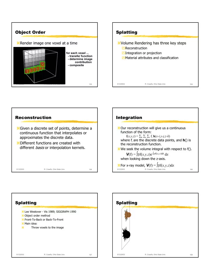
Object Order

Render image one voxel at a time

for each voxel ...

• transfer function
• determine image

contribution

• composite

5/12/2003

• R. Crawfis, Ohio State Univ.

104

Splatting

Volume Rendering has three key steps

Reconstruction Integration or projection Material attributes and classification

5/12/2003

• R. Crawfis, Ohio State Univ.

105

Reconstruction

Given a discrete set of points, determine a continuous function that interpolates or approximates the discrete data. Different functions are created with different basis or interpolation kernels.

5/12/2003

• R. Crawfis, Ohio State Univ.

106

Integration

Our reconstruction will give us a continuous function of the form: f(x,y,z) = ∑k ∑j ∑i fi h(x-i,y-j,z-k) where fi are the discrete data points, and h() is the reconstruction function. We seek the volume integral with respect to f().

V(f) = ∫βf(x,y,z)e-∫ρf(x,y,t)dt dz

when looking down the z-axis. For x-ray model, V(f) = ∫βf(x,y,z)dz

5/12/2003

• R. Crawfis, Ohio State Univ.

107

Splatting

Lee Westover - Vis 1989; SIGGRAPH 1990 Object order method Front-To-Back or Back-To-Front Main idea:

• Throw voxels to the image

5/12/2003

• R. Crawfis, Ohio State Univ.

108

Splatting

SLIDE 2

2

5/12/2003

• R. Crawfis, Ohio State Univ.

109

Splatting

Process from closest voxel to furthest voxel Biggest problem: determination of voxel’s projected area called its footprint

5/12/2003

• R. Crawfis, Ohio State Univ.

110

Splatting Algorithm:

• 5/12/2003
• R. Crawfis, Ohio State Univ.

111

Splatting

Volume = field of 3D interpolation kernels

One kernel at each grid voxel

Each kernel leaves a 2D footprint on screen

Voxel contribution = footprint ·(C, opacity)

Weighted footprints accumulate into image

voxel kernels screen footprints = splats screen

5/12/2003

• R. Crawfis, Ohio State Univ.

112

Splatting

Volume = field of 3D interpolation kernels

One kernel at each grid voxel

Each kernel leaves a 2D footprint on screen

Voxel contribution = footprint ·(C, opacity)

Weighted footprints accumulate into image

voxel kernels screen footprints = splats screen

5/12/2003

• R. Crawfis, Ohio State Univ.

113

Splatting

Volume = field of 3D interpolation kernels

One kernel at each grid voxel

Each kernel leaves a 2D footprint on screen

Voxel contribution = footprint ·(C, opacity)

Weighted footprints accumulate into image

voxel kernels screen footprints = splats screen

5/12/2003

• R. Crawfis, Ohio State Univ.

114

Splatting

Volume = field of 3D interpolation kernels

One kernel at each grid voxel

Each kernel leaves a 2D footprint on screen

Voxel contribution = footprint ·(C, opacity)

Weighted footprints accumulate into image

voxel kernels screen footprints = splats screen

SLIDE 3

3

5/12/2003

• R. Crawfis, Ohio State Univ.

115

Ray-casting - revisited

color c = c s αs(1 - α) + c

• pacity α = α s (1 - α) + α

1.0

• bject (color, opacity)

volumetric compositing Interpolation kernel

5/12/2003

• R. Crawfis, Ohio State Univ.

116

Ray-casting - revisited

(ideally) we would reconstruct the continuous volume (cloud) using the interpolation kernel h: the we would compute the analytic integral along a ray r: this can only be approximated by discretization

( ) ( )

∫∑ ∫

− + = + =

k k k r

dr v f v r p h dr r p f p I ) ( ) (

∑

− =

k k k r

v f v v h v f ) ( ) ( ) (

5/12/2003

• R. Crawfis, Ohio State Univ.

117

( ) ( )

∑ ∫

− + =

k k k

dr v r p h v f p I ) (

Splatting - principal idea

This last equation can be rewritten in the following way:

( ) ( )

∫∑

− + =

k k k

dr v f v r p h p I ) (

Splatting Kernel or “Splat”

Which can be computed analytically

analytically: known as footprint

( )dz

z y x h y x

∫

= , , ) , ( Splat

5/12/2003

• R. Crawfis, Ohio State Univ.

118

Footprint Extent

Approximate the 3D kernel (h(x,y,z))extent by a sphere

5/12/2003

• R. Crawfis, Ohio State Univ.

119

3D kernel

x filter extent y filter extent Image-space splat coordinate pixels Filter footprint Filter kernel

Positioning each splat on the screen and compositing the contribution into each pixel

5/12/2003

• R. Crawfis, Ohio State Univ.

120

Integrate to footprint table

3D filter kernel Integrate along one dimension 2D filter kernel The 3D rotationally symmetric filter kernel is integrated to produce a 2D filter kernel

SLIDE 4

4

5/12/2003

• R. Crawfis, Ohio State Univ.

121

Footprint Table

A popular kernel is a three-dimensional Gaussian (radially symmetric) As 1D integration of 3D Gaussian is still a 2D Gaussian – we can just skip the Z integration and evaluate the Gaussian function on 2D image space after voxel projection Generic footprint table

preprocessing

5/12/2003

• R. Crawfis, Ohio State Univ.

122

Overlapping Problem

Splat 1 Splat 2 Desired result

5/12/2003

• R. Crawfis, Ohio State Univ.

123

Overlapping Problem

Splat 1 Splat 2 Actual result

5/12/2003

• R. Crawfis, Ohio State Univ.

124

View-dependent footprint

It is possible to transform a sphere kernel into A ellipsoid

• The projection of an

ellipsoid is an ellipse

• We need to transform the

generic footprint table to the ellipse

5/12/2003

• R. Crawfis, Ohio State Univ.

125

View-dependent footprint (2)

5/12/2003

• R. Crawfis, Ohio State Univ.

126

Example Footprint at Different Resolutions

SLIDE 5

5

5/12/2003

• R. Crawfis, Ohio State Univ.

127

Footprint - principal idea

Draw each voxel as a cloud of points (footprint) that spreads the voxel contribution across multiple pixels. Larger footprint -> larger spatial kernel extent -> lower frequency components -> more blurring

Large pixel/voxel ratio

5/12/2003

• R. Crawfis, Ohio State Univ.

128

Rendering a Splat

Use texture mapping hardware to resample footprint table (either single density channel or separate classified r,g,b,a channels)

5/12/2003

• R. Crawfis, Ohio State Univ.

129

Splatting: Original Implementation

voxels

Volume

sheet buffer compositing buffer image plane

5/12/2003

• R. Crawfis, Ohio State Univ.

130

Splatting: Original Implementation

voxels Rasterization image plane

Add voxel kernels within first sheet

5/12/2003

• R. Crawfis, Ohio State Univ.

131

Splatting: Original Implementation

voxels image plane

Add voxel kernels to the image.

5/12/2003

• R. Crawfis, Ohio State Univ.

132

Splatting: Original Implementation

voxels image plane

Add voxel kernels to the image.

SLIDE 6

6

5/12/2003

• R. Crawfis, Ohio State Univ.

133

Splatting: Original Implementation

voxels image plane

Add voxel kernels to the image.

5/12/2003

• R. Crawfis, Ohio State Univ.

134

Splatting: Second Implementation

voxels

Do for all voxels in some bak-to-front order.

image plane

5/12/2003

• R. Crawfis, Ohio State Univ.

135

Splatting - efficiency

“footprint” - splatted (integrated) kernel if interpolation kernel is radially symmetric (spherical) then its footprint is independent of the view point (for orthographic viewing) for perspective - footprint can be approximated with an ellipse Hence, for common cases, we can pre-integrate it (efficient!) for perspective projection, to approximate, we have to compute the orientation of the ellipse

5/12/2003

• R. Crawfis, Ohio State Univ.

136

Splatting - Highlights

Footprints can be pre-integrated

fast voxel projection

Advantages over ray-casting:

Fast: voxel interpolation is in 2D on screen More accurate integration (analytic for X-ray) More accurate reconstruction (afford better kernels) Only relevant voxels must be projected

5/12/2003

• R. Crawfis, Ohio State Univ.

137

Early Implementation – Axis

Aligned Splatting

Voxel kernels are added within axis-aligned sheets Sheets are composited front-to-back Sheets = volume slices most perpendicular to the image plane

image plane at 70° image plane at 30° volume slices

x y z

volume slices

5/12/2003

• R. Crawfis, Ohio State Univ.

138

Splatting: Highlights

Footprints can be pre-integrated

fast voxel projection

Advantages over raycasting:

Fast: voxel interpolation is in 2D on screen More accurate integration

⌧analytical for X-ray

More accurate reconstruction

⌧afford better kernels

Only relevant voxels must be projected

SLIDE 7

7

5/12/2003

• R. Crawfis, Ohio State Univ.

139

Splatting: Second Implementation

Voxel kernels are added within sheets Sheets are composited front-to-back Sheets = volume slices most perpendicular to the image plane

image plane at 70° volume slices image plane at 30° volume slices

x y z

5/12/2003

• R. Crawfis, Ohio State Univ.

140

Splatting: Second Implementation

sheet buffer compositing buffer volume slices image plane

Volume

5/12/2003

• R. Crawfis, Ohio State Univ.

141

Splatting: Second Implementation

sheet buffer compositing buffer volume slices image plane Add voxel kernels within first sheet to an auxillary buffer.

5/12/2003

• R. Crawfis, Ohio State Univ.

142

Splatting: Second Implementation

sheet buffer compositing buffer volume slices image plane

Transfer to the compositing buffer

5/12/2003

• R. Crawfis, Ohio State Univ.

143

Splatting: Second Implementation

sheet buffer compositing buffer volume slices image plane

Add voxel kernels within second sheet

5/12/2003

• R. Crawfis, Ohio State Univ.

144

Splatting: Second Implementation

sheet buffer compositing buffer volume slices image plane

Composite sheet under the compositing buffer

SLIDE 8

8

5/12/2003

• R. Crawfis, Ohio State Univ.

145

Splatting: Second Implementation

sheet buffer compositing buffer volume slices image plane

Add voxel kernels within third sheet

5/12/2003

• R. Crawfis, Ohio State Univ.

146

Splatting: Second Implementation

sheet buffer compositing buffer volume slices image plane

Composite sheet with compositing buffer

5/12/2003

• R. Crawfis, Ohio State Univ.

147

Splatting – Second Implementation Artifacts

At 45°, popping occurs:

44.7° 45.2° binary cube

5/12/2003

• R. Crawfis, Ohio State Univ.

148

Cube Viewed at 45°

color buffer binary cube

5/12/2003

• R. Crawfis, Ohio State Univ.

149

Cube Viewed at 45°

color buffer binary cube

5/12/2003

• R. Crawfis, Ohio State Univ.

150

Cube Viewed at 45°

color buffer binary cube

SLIDE 9

9

5/12/2003

• R. Crawfis, Ohio State Univ.

151

Cube Viewed at 45°

color buffer binary cube

5/12/2003

• R. Crawfis, Ohio State Univ.

152

Cube Viewed at 45°

color buffer binary cube

5/12/2003

• R. Crawfis, Ohio State Univ.

153

Cube Viewed at 45°

color buffer binary cube

5/12/2003

• R. Crawfis, Ohio State Univ.

154

Cube Viewed at 45°

color buffer binary cube

5/12/2003

• R. Crawfis, Ohio State Univ.

155

Cube Viewed at 45°

color buffer binary cube

5/12/2003

• R. Crawfis, Ohio State Univ.

156

Cube Viewed at 45°

color buffer binary cube

SLIDE 10

10

5/12/2003

• R. Crawfis, Ohio State Univ.

157

Cube Viewed at 45.1°

color buffer binary cube

5/12/2003

• R. Crawfis, Ohio State Univ.

158

Cube Viewed at 45.1°

color buffer binary cube

5/12/2003

• R. Crawfis, Ohio State Univ.

159

Cube Viewed at 45.1°

color buffer binary cube

5/12/2003

• R. Crawfis, Ohio State Univ.

160

Cube Viewed at 45.1°

color buffer binary cube

5/12/2003

• R. Crawfis, Ohio State Univ.

161

Cube Viewed at 45.1°

color buffer binary cube

5/12/2003

• R. Crawfis, Ohio State Univ.

162

Cube Viewed at 45.1°

color buffer binary cube

SLIDE 11

11

5/12/2003

• R. Crawfis, Ohio State Univ.

163

Cube Viewed at 45.1°

color buffer binary cube

5/12/2003

• R. Crawfis, Ohio State Univ.

164

Cube Viewed at 45.1°

color buffer binary cube

5/12/2003

• R. Crawfis, Ohio State Univ.

165

Cube Viewed at 45.1°

color buffer binary cube

5/12/2003

• R. Crawfis, Ohio State Univ.

166

adding: (c1+c2) (α1 + α2) compositing: c2 α2 (1-α1) + c1α1 >

Adding vs. Compositing

Added color > composited color

5/12/2003

• R. Crawfis, Ohio State Univ.

167

Comparison

interpolated slices are aligned with image plane voxels spread energy into several slices

interpolated slices (C, α) image plane c

• m

p

• s

i t e

voxels add all energy into one sheet Slice-interpolation method sheet buffers are aligned with a volume plane Splatting

5/12/2003

• R. Crawfis, Ohio State Univ.

168

Apply Slice-Interpolation Model To Splatting

In raycasting:

Volume is an array of discrete points Discrete volume data points support 3D interpolation

New scenario for splatting:

Volume is array of overlapping kernels Interpolation planes chop kernels into slices All kernel material between planes must be added into sheet- buffer before compositing

SLIDE 12

12

5/12/2003

• R. Crawfis, Ohio State Univ.

169

Image-Aligned Sheet-Buffer

sheet buffer compositing buffer

Slicing slab cuts kernels into sections Kernel sections are added into sheet- buffer Sheet-buffers are composited

image plane

5/12/2003

• R. Crawfis, Ohio State Univ.

170

Image-Aligned Sheet-Buffer

sheet buffer compositing buffer

Slicing slab cuts kernels into sections Kernel sections are added into sheet- buffer Sheet-buffers are composited

image plane

5/12/2003

• R. Crawfis, Ohio State Univ.

171

Image-Aligned Sheet-Buffer

sheet buffer compositing buffer

Slicing slab cuts kernels into sections Kernel sections are added into sheet- buffer Sheet-buffers are composited

image plane

5/12/2003

• R. Crawfis, Ohio State Univ.

172

Image-Aligned Sheet-Buffer

sheet buffer compositing buffer

Slicing slab cuts kernels into sections Kernel sections are added into sheet- buffer Sheet-buffers are composited

image plane

5/12/2003

• R. Crawfis, Ohio State Univ.

173

Image-Aligned Sheet-Buffer

sheet buffer compositing buffer

Slicing slab cuts kernels into sections Kernel sections are added into sheet- buffer Sheet-buffers are composited

image plane

5/12/2003

• R. Crawfis, Ohio State Univ.

174

Image-Aligned Sheet-Buffer

sheet buffer compositing buffer

Slicing slab cuts kernels into sections Kernel sections are added into sheet- buffer Sheet-buffers are composited

image plane

SLIDE 13

13

5/12/2003

• R. Crawfis, Ohio State Univ.

175

Image-Aligned Sheet-Buffer

sheet buffer compositing buffer

Slicing slab cuts kernels into sections Kernel sections are added into sheet- buffer Sheet-buffers are composited

image plane

5/12/2003

• R. Crawfis, Ohio State Univ.

176

Results: Ganglion Nerve Cell

44.2° 44.7° 45.2° axis- aligned movie image- aligned movie

5/12/2003

• R. Crawfis, Ohio State Univ.

177

Kernel-Slice Footprint Array

Kernels are sliced into sections:

need to supply slice footprints → footprint array

slab width kernel slice footprint array …..

5/12/2003

• R. Crawfis, Ohio State Univ.

178

Image-Aligned Splatting

Note: We need an array of footprint tables

• now. A separate footprint table for each slice
• f the 3D reconstruction kernel.

5/12/2003

• R. Crawfis, Ohio State Univ.

179

Image-Aligned Splatting: Highlights

Similar to ideal slice-interpolation method and raycasting In addition, it offers:

analytical kernel slice integration efficient use of high-quality interpolation kernels

Downside: Need more footprint projections

but rasterization coherencies can be exploited

Accuracy / speed controllable via slice width

5/12/2003

• R. Crawfis, Ohio State Univ.

180

Volume Rendering Pipeline: Two Variations

SLIDE 14

14

5/12/2003

• R. Crawfis, Ohio State Univ.

181

Volume Rendering Pipeline: Two Variations

5/12/2003

• R. Crawfis, Ohio State Univ.

182

IASB Splatting

No popping or color bleeding Sharp, noise-free images

5/12/2003

• R. Crawfis, Ohio State Univ.

183

Efficiency Considerations

Splatting

✗ splat all relevant voxels, even if invisible

Raycasting

✓ stop ray when

• paque (early ray

termination) Would like early splat elimination for Splatting

5/12/2003

• R. Crawfis, Ohio State Univ.

184

Occlusion Culling

A voxel is only visible if the volume material in front is not opaque

• ccluded voxel: does not

pass visibility test wall of occluding voxels

• cclusion map = opacity image

screen

5/12/2003

• R. Crawfis, Ohio State Univ.

185

Visibility Test Based on Occlusion Buffer

• pacity ≥ threshold
• cclusion map

Do not project Project

• pacity < threshold
• pacity = 0

Compute occlusion map after each sheet Cull both individual voxel and voxel sets using an occlusion map

5/12/2003

• R. Crawfis, Ohio State Univ.

186

Early Splat Elimination - Results

standard early elim. voxels splatted Head (2563) 54.6 s 12.7 s 3 %

• Transp. head

35.8 s 14.8 s 21 % Nerve (512x76) 17.6 s 8.4 s 10 % Tomato (2563) 36.8 s 15.5 s 37 %

SLIDE 15

15

5/12/2003

• R. Crawfis, Ohio State Univ.

187

Perspective Projection

Adds realism

human visual system uses perspective provides depth cues

5/12/2003

• R. Crawfis, Ohio State Univ.

188

Perspective Volume Grid Sampling

Back regions of grid are undersampled

Ray grid sampling rate > volume grid sampling rate → no aliasing Ray grid sampling rate ≤ volume grid sampling rate → aliasing screen

• versampled

volume grid undersampled volume grid

5/12/2003

• R. Crawfis, Ohio State Univ.

189

Effects of Aliasing

checkerboard tunnel terrain movie

5/12/2003

• R. Crawfis, Ohio State Univ.

190

Perspective Volume Grid Sampling

Need to low-pass undersampled regions

Ray grid sampling rate > volume grid sampling rate → no aliasing Ray grid sampling rate ≤ volume grid sampling rate → aliasing screen low-pass use as is

5/12/2003

• R. Crawfis, Ohio State Univ.

191

Anti-Aliased Splatting

Splatting offers elegant, on-the-fly solution:

screen linearly increase splat kernel size constant splat kernel size

IEEE Trans. Vis. and Comp. Graph. ‘98

5/12/2003

• R. Crawfis, Ohio State Univ.

192

Results: Checkerboard Tunnel

aliased anti-aliased

SLIDE 16

16

5/12/2003

• R. Crawfis, Ohio State Univ.

193

Results: Perspective Terrain Rendering

aliased anti-aliased movie

5/12/2003

• R. Crawfis, Ohio State Univ.

194

Post-Reconstruction Classification

5/12/2003

• R. Crawfis, Ohio State Univ.

195

Post-Reconstruction Classification

5/12/2003

• R. Crawfis, Ohio State Univ.

196

Post-Reconstruction Classification

5/12/2003

• R. Crawfis, Ohio State Univ.

197

Lighting and Shading

Functional or distance reconstruction allows for high-quality normal calculation This can be done in a post-reconstruction mode as well, allowing for per-pixel normals. This allows for Phong shading.

5/12/2003

• R. Crawfis, Ohio State Univ.

198

Anti-aliasing

Needed to preserve small features Needed for the diverging rays in perspective

Aliased anti-aliased

SLIDE 17

17

5/12/2003

• R. Crawfis, Ohio State Univ.

199

Amorphous Phenomena

Rather than modulate or texture map each pixel, pre-map the splats.

5/12/2003

• R. Crawfis, Ohio State Univ.

200

Fire

Volume rendering with traditional splatting (left) Volume rendering with textured splats (right)

5/12/2003

• R. Crawfis, Ohio State Univ.

201

Fast Animation of Fire

Add detail to footprint, creating a splat that contains high frequency information. Rendering with these splats creates fast animation with detail. Cycling splats creates inter- and intra-voxel dynamics

5/12/2003

• R. Crawfis, Ohio State Univ.

202

Amorphous Phenomena