electron crystallography of two dimensional crystals
play

Electron Crystallography of Two-Dimensional Crystals The Basics V. - PDF document

Negative Stain Image of 2D-Crystal Electron Crystallography of Two-Dimensional Crystals The Basics V. Unger, 11/4/2005 To grasp the basic ideas underlying electron crystallographic image processing, all we need to ask is: how can we


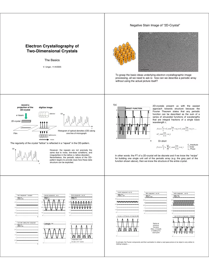
  1. Negative Stain Image of “2D-Crystal” Electron Crystallography of Two-Dimensional Crystals The Basics V. Unger, 11/4/2005 To grasp the basic ideas underlying electron crystallographic image processing, all we need to ask is: how can we describe a periodic array without using the actual picture itself? f(x) record a 2D-crystals present us with the easiest projection of the digitize image approach towards structure because the TARGET FUNCTION 2D-crystal 4 Fourier Theorem states that any periodic detector function can be described as the sum of a OD e - -beam series of sinusoidal functions of wavelengths 3 that are integral fractions of a single basic 2D-crystal wavelength � . 2 f ( x ) = C 0 + C 1 cos(2 � x + � 1 ) + C 2 cos(2 � x x + � 2 ) + .... Histogram of optical densities (OD) along � � /2 2 1 Film one line of micrograph + C n cos(2 � x + � n ) lightsource � / n 0 move x Or short The regularity of the crystal “lattice” is reflected in a “repeat” in the OD-pattern. C n Amplitude n = � f ( x ) = C 0 C n cos(2 � x � n Order � / n + � n ) 2 + OD � n Phase However: the repeats are not precisely the n = 1 same due to noise, low-dose conditions, and irregularities in the lattice (= lattice disorder). In other words: the FT of a 2D-crystal will be discrete and if we know the “recipe” Nevertheless, the periodic nature of the OD- for building one single unit cell of the periodic array (e.g. the grey part of the pattern begins to provide clues how these data function shown above), then we know the structure of the entire crystal. structure can be exploited. x 2 fourth component: cos 3x 2 2 1.5 fifth component: cos 4x sixth component: cos 5x 4 2 2 Amp = 0.1 1.5 1.5 second component: cos x third component: cos 2x first component: constant Phase = -135˚ Amp = 0 Amp = 0.5 1 Phase = any Phase = 90˚ 3.5 1.5 1.5 Amp = 0.7 1 1 Amp = 2 Amp =1 phase: any Phase = 0˚ Phase = 0˚ 0.5 1 1 3 0.5 0.5 0 0.5 0.5 2.5 0 0 -0.5 2 0 0 -0.5 -0.5 -1 1.5 -0.5 -0.5 -1 -1 -1.5 1 -1 -1 -1.5 -1.5 -2 0.5 -1.5 -1.5 -2 -2 -2 0 -2 2+ cos x + 0.7*cos 2x + 0.1*cos (3x-135) sum of all six components = TARGET X 4 4 4 3 3 sum after adding first component Same as 4 component 1+2 4 3.5 = 2 + cos x Amp = 2 previous phase: any 2 because 3 2 Amp = 0 results 3 3 2.5 in adding 0 to 1 1 each point 2 2 2 1.5 0 0 1 1 1 components 1+2+3 0.5 In principle: the Fourier components and their summation to obtain a real space picture of an object is very similar to 2+ cos x + 0.7 * cos 2x 0 0 0 making Lasagna…. X

  2. To prove the point…. Principle of Digital Filtering (0,5) (4,2) (5,0) (0,0) cryoEM picture of a gap junction 2D- crystal (periodic object) deposited on Calculated FT of the image. What do continuous carbon support film you see? And what is causing it? circular maskholes entire FT (aperiodic object) enlarged area of FT applied (FT has now non-zero Spots at regular spacings: diffraction maxima arising from crystal . a) values only within b) Alternating pattern of bright and dark regions. This is a combination of two things. (1) the aperiodic carbon film causes diffraction at all angles , and (2) the oscillation in intensities maskholes is the manifestation of the CTF of the objective lens (not all diffracted waves are transmitted with the same fidelity) Digital Filtering of Fourier Transform Digital Filtering of Fourier Transform Radius used was r=1 Radius used was r=7 origin autocorrelation Autocorrelation Map Part of Crosscorrelation Map c(x) 1 two copies of x w same object -w w 0 x 0 crosscorrelation c(x) 1 two similar objects -w w x � x c(x) � x 1 two identical objects with translational Note that the shape of the central peak in the autocorrelation map is very offset -w w x similar to the shape of the cross-correlation peaks.

  3. Crosscorrelation Maps Effect of “Lattice Unbending” Cross-correlation methods can be used to determine translational disorder in 2D-crystals. 7Å 10Å 15Å 7Å 10Å 15Å Left: data were retrieved from a Right: after correction for calculated FT of an untreated raw translational lattice disorder, the image. In this case, the data are not same image provides data out to statistically significant beyond ~15Å ~7Å resolution. deviation from expected lattice height of cross correlation-peaks indicates resolution. position [Å] X20 (not to scale) with how similar each unit cell is to the chosen Plot symbols indicate the goodness of each reflection. Reflections marked by a “1” respect to chosen reference reference have a signal-to-noise ratio of at least 8. Because the phase information is so important we now can Now that the data extend to well beyond 10Å, correction for the CTF understand why in EM we MUST correct for the effect of the becomes critically important. CTF…. Reciprocal space The simulated curves are for 3000 and 6000Å of underfocus respectively, an accelerating voltage of 200keV ( � =0.025Å) and Inverse FT = a C s =2mm F hk Amplitude of reflection (h,k) Fourier These lower two panels � � F hk e i � hk e � 2 � i ( hx + ky ) f ( x , y ) = � hk Phase of reflection (h,k) Summation demonstrate how the CTF would h k look like in the FT of the image. Circles represent [sin � ( � )] =0 Frequencies where [sin � ( � )]<0 contribute with reversed contrast to CTF- the image. Therefore, the phases Real correction space of reflections in these regions need to be adjusted by 180˚ REAL SPACE RECIPROCAL SPACE Basic Image Processing of 2D-Crystals FT of Raw Image DIGITIZED RAW IMAGE Digitally Filtered Image (H,K) amp phase IQ CTF (small radius) 0 1 132.4 237.8 7 -0.142 0 2 5686.9 299.8 1 -0.540 Masked FT of 0 3 195 249.1 6 -0.958 FT of Reference Raw Image Reference Area 0 4 1067.4 246.1 1 -0.762 (large radius) 0 5 431.0 102.5 2 0.397 0 6 1016.5 356.5 1 0.925 0 7 120.5 243.0 6 -0.602 Crosscorrelation Autocorrelation 0 8 0.0 270.7 9 -0.388 FT of CC-Map Map Map 0 9 145.5 319.4 4 0.923 0 10 67.2 290.6 6 -0.993 0 11 0.0 270.7 9 0.928 List of CC-peaks 1 0 97.7 132.8 8 -0148 1 1 7227.8 140.0 1 -0.423 1 2 2582.2 17.1 1 -0.846 Reinterpolated “Unbent” Image 1 3 1460.3 266.5 1 -0.957 And so forth…. LIST OF AMPLITUDES AND Boxed and “Unbent” Image RECIPROCAL SPACE PHASES REAL SPACE

Download Presentation
Download Policy: The content available on the website is offered to you 'AS IS' for your personal information and use only. It cannot be commercialized, licensed, or distributed on other websites without prior consent from the author. To download a presentation, simply click this link. If you encounter any difficulties during the download process, it's possible that the publisher has removed the file from their server.

Recommend


More recommend