Einfhrung in Visual Computing U it 14 Gl b l O Unit 14: Global - - PowerPoint PPT Presentation

Einführung in Visual Computing

U it 14 Gl b l O ti Unit 14: Global Operations

http://www.caa.tuwien.ac.at/cvl/teaching/sommersemester/evc

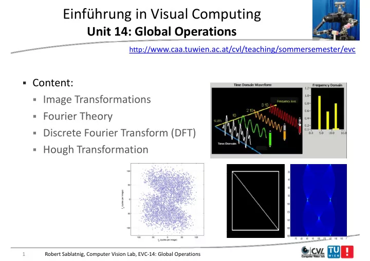
• Content:
• Image Transformations
• Fourier Theory
• Fourier Theory
• Discrete Fourier Transform (DFT)
• Hough Transformation

1 Robert Sablatnig, Computer Vision Lab, EVC‐14: Global Operations

Increasing frequency Increasing frequency

Image Transformations

Why transform Data y

• To de

de‐correlate correlate data so that fast scalar (rather than slow vector) quantization can be used q

• To exploit better the characteristics of the Human Visual System

Human Visual System (HVS) by separating the data into vision vision‐sensitive parts sensitive parts and (HVS) by separating the data into vision vision sensitive parts sensitive parts and vision‐insensitive parts.

• To compact

compact most of the ”energy energy” in a few coefficients so that to

• To compact

compact most of the energy energy in a few coefficients, so that to discard most of the coefficients and thus achieve compression

3 Robert Sablatnig, Computer Vision Lab, EVC‐14: Global Operations

Transforms

• Various transforms achieve those properties to various extents
• Discrete Fourier Transform (DFT)
• Discrete Fourier Transform (DFT)
• Discrete Cosine Transform (DCT)

Oth F i lik t f

• Other Fourier‐like transforms:

Haar, Walsh, Hadamard

• Karhunen‐Loeve Transform (KLT)
• Discrete Wavelet Transforms (DWT)

( )

4 Robert Sablatnig, Computer Vision Lab, EVC‐14: Global Operations

Matrix Formulation of Transform

• Transform is a matrix multiplication of the input signal and the

transform‐matrix .

• The standard transform is defined by an N×N square matrix AN.

The standard transform is defined by an N×N square matrix AN.

• Transform of a 1D discrete input signal (a column vector x of N
• Transform of a 1D discrete input signal (a column vector x of N

components) y = y = ANx

5 Robert Sablatnig, Computer Vision Lab, EVC‐14: Global Operations

Transform

• Transform of an N×N image X is a transform of each column

followed by transform of each row (separable transform separable transform) y ( p ) In matrix form, transform of image X is the computation of: y = y = A XA XA t y = y = ANXA XAN

t

• The inverse transform is x =

x = BNy for 1D signals, and X = X = BNYB YBN

t for

images , where t is the transposed matrix, and BN = A = A‐1

1

6 Robert Sablatnig, Computer Vision Lab, EVC‐14: Global Operations

Orthonormal Transforms

• Thus, the inverse transform is

x = A x = AN

‐1y for 1D signals, 1 1 ( 1 1)t

A-1= AT

AAT I

and X = A X = AN

‐ ‐1 1 Y(A

Y(AN

‐ ‐1 1)t t for images

AAT= I

Basis vectors

7 Robert Sablatnig, Computer Vision Lab, EVC‐14: Global Operations

Orthonormal Transforms

Fo rier Fourier

Fourier Theory

Fourier Transform

• Property of transforms:
• They convert a function from one domain to another with no
• They convert a function from one domain to another with no

loss of information

• Fourier Transform:
• Fourier Transform:

dt t G

x i



  

) ( 1 ) ( dt e t g G

x i



 

 



  ) ( 2 ) (

converts a function from the spatial (or time) domain to the frequency domain

10 Robert Sablatnig, Computer Vision Lab, EVC‐14: Global Operations

Time Domain and Frequency Domain q y

• Time Domain:
• Tells us how properties (air pressure in a sound function, for

p p ( p , example) change over time: Amplitude = 100 Amplitude = 100 Frequency = number of cycles in one second = 200 Hz

11 Robert Sablatnig, Computer Vision Lab, EVC‐14: Global Operations

Time Domain and Frequency Domain q y

• Frequency domain:
• Tells us how properties (amplitudes) change over frequencies:
• Tells us how properties (amplitudes) change over frequencies:

12 Robert Sablatnig, Computer Vision Lab, EVC‐14: Global Operations

Time Domain and Frequency Domain q y

• Example:
• Human ears do not hear wave‐like oscilations but constant
• Human ears do not hear wave like oscilations, but constant

tone

• Often it is easier to work in the frequency domain

13 Robert Sablatnig, Computer Vision Lab, EVC‐14: Global Operations

A Sine Wave

8 4 6

5*sin (24t) Amplitude = 5

2

Frequency = 4 Hz

• 2

We take an ideal sine wave

• 6
• 4

to discuss effects of sampling

0.1 0.2 0.3 0.4 0.5 0.6 0.7 0.8 0.9 1

• 8

seconds

sampling

seconds

14 Robert Sablatnig, Computer Vision Lab, EVC‐14: Global Operations

A sine Wave Signal g

6 8

5*sin(24t)

4 6

Amplitude = 5 Frequency = 4 Hz

2

Frequency = 4 Hz Sampling rate = 256 samples/second

• 4
• 2

sa p es/seco d Sampling duration = 1 second

0.1 0.2 0.3 0.4 0.5 0.6 0.7 0.8 0.9 1

• 8
• 6

We do sampling of 4Hz signal with 256 Hz so

seconds

sampling is in much higher rate than the base frequency, good

Thus after sampling we can reconstruct the original signal

Robert Sablatnig, Computer Vision Lab, EVC‐14: Global Operations 15

frequency, good

An undersampled Signal p g

Here sampling rate is 8.5 Hz and the frequency is 8 Hz

2

sin(28t), SR = 8.5 Hz

1 1.5 0.5

• 0.5

Undersampling can be confusing H it t

• 1.5
• 1

Here it suggests a different frequency of

0.2 0.4 0.6 0.8 1 1.2 1.4 1.6 1.8 2

• 2

sampled signal

16 Robert Sablatnig, Computer Vision Lab, EVC‐14: Global Operations

The Nyquist Frequency yq q y

• The Nyquist frequency is equal to one‐half of the sampling

frequency. q y

• The Nyquist frequency is the highest frequency that can be

measured in a signal. measured in a signal.

Nyquist invented method to have a d l f good sampling frequency

17 Robert Sablatnig, Computer Vision Lab, EVC‐14: Global Operations

Time Domain and Frequency Domain q y

• In 1807, Jean Baptiste Joseph Fourier showed that any periodic

signal could be represented by a series of sinusoidal functions g p y

the composition of the first two functions gives the bottom one

18 Robert Sablatnig, Computer Vision Lab, EVC‐14: Global Operations

Fourier Transform

• A Fourier Transform is an integral transform

integral transform that re‐expresses a function in terms of different sine waves different sine waves of varying amplitudes amplitudes, y g p , wavelengths wavelengths, and phases phases.

• So what does this mean exactly?

So what does this mean exactly?

Can be represented by: Let’s start with an example…in 1‐D When you let these three waves interfere with each other you get your

• riginal wave function!

19 Robert Sablatnig, Computer Vision Lab, EVC‐14: Global Operations

Time Domain and Frequency Domain q y

20 Robert Sablatnig, Computer Vision Lab, EVC‐14: Global Operations

Famous Fourier Transforms

2 1

Sine wave

0.2 0.4 0.6 0.8 1 1.2 1.4 1.6 1.8 2

• 2
• 1

In time In time

200 250 300 50 100 150

Delta function In frequency In frequency

20 40 60 80 100 120

21 Robert Sablatnig, Computer Vision Lab, EVC‐14: Global Operations

Famous Fourier Transforms

0.5 0.2 0.3 0.4

Gaussian

5 10 15 20 25 30 35 40 45 50 0.1

In time In time

4 5 6 1 2 3 4

Gaussian In frequency In frequency

50 100 150 200 250

22 Robert Sablatnig, Computer Vision Lab, EVC‐14: Global Operations

Famous Fourier Transforms

1.5 0.5 1

Sinc function

• 1
• 0.8
• 0.6
• 0.4
• 0.2

0.2 0.4 0.6 0.8 1

• 0.5

In time In time

4 5 6 1 2 3 4

Square wave In frequency In frequency

• 100
• 50

50 100

23 Robert Sablatnig, Computer Vision Lab, EVC‐14: Global Operations

Famous Fourier Transforms

1.5

Sinc function

0.5 1

• 1
• 0.8
• 0.6
• 0.4
• 0.2

0.2 0.4 0.6 0.8 1

• 0.5

In time In time

4 5 6

Square wave

1 2 3 4

In frequency In frequency

• 100
• 50

50 100

24 Robert Sablatnig, Computer Vision Lab, EVC‐14: Global Operations

Fourier Transform

• Since this object can be made up of 3 fundamental frequencies an

ideal Fourier Transform would look something like this:

Increasing Frequency Increasing Frequency

• Notice that it is symmetric around the central point and that the

g q y g q y

amount of points radiating outward correspond to the distinct frequencies used in creating the image.

25 Robert Sablatnig, Computer Vision Lab, EVC‐14: Global Operations

Let’s Try it with Two‐Dimensions! y

This image exclusively has 32 cycles in vertical direction. This image exclusively has 8 cycles in horizontal direction.

You will notice that the second example is a little more smeared

• ut. This is because the lines are more blurred so more sine waves

are required to build it. The transform is weighted so brighter spots indicate sine waves more frequently used. q y

26 Robert Sablatnig, Computer Vision Lab, EVC‐14: Global Operations

So what is going on here? g g

Th i f l ft t i ht d t th h i t l

• The u axis runs from left to right and represents the horizontal

component of the frequency. The v axis runs up and down and corresponds to vertical components of the frequency corresponds to vertical components of the frequency.

x‐y coordinate system Fourier Transform

Th t l d t i f ll i it i ll

u‐v coordinate system

• The central dot is an average of all sine waves so it is usually

brightest dot and used as point of reference for the rest Si hi i i d l h i i ill b f h

• Since this is inverse space, dots close to the origin will be further

apart in real space than dots that are far apart on the Fourier Transform (these dots refer to the frequency of a component wave )

• Transform. (these dots refer to the frequency of a component wave.)

Robert Sablatnig, Computer Vision Lab, EVC‐14: Global Operations 27

Again… g

This image exclusively has 4 cycles horizontally and 16 cycles vertically This image exclusively has 32 cycles horizontally and 2 cycles vertically horizontally and 16 cycles vertically horizontally and 2 cycles vertically

• If the image is symmetrical across the x‐axis in real space then it

will also be in inverse space will also be in inverse space.

28 Robert Sablatnig, Computer Vision Lab, EVC‐14: Global Operations

Fourier Transform

• Because of the property: eiθ = cosθ + i sinθ

eiωt= cos ωt + i sin ωt

Eulers Formula

where

1   i

Fourier Transform takes us to the frequency domain:

Sinusoidal varying

 

dt t f F

t i





 

) ( 1

„basis“ function for the expansion

 

dt e t f F

t i



 





  ) ( 2

The Fourier transform; Scale factor for the Fourier Transform F(ω); The Fourier transform; strength of frequency ω contained in f(t) Scale factor for the Fourier Transform F(ω); the original signal in the time domain; the „inverse Fourier Transform“.

29 Robert Sablatnig, Computer Vision Lab, EVC‐14: Global Operations

2D Sinusoids:

c

( )

... are plane waves with grayscale amplitudes, periods in t f l th

c

• rientation
• rientation

terms of lengths, ...



r

A  = phase shift

Robert Sablatnig, Computer Vision Lab, EVC‐14: Global Operations 30

2D Sinusoids:

specific orientations ... specific orientations, and phase shifts.

c c r r r r

Robert Sablatnig, Computer Vision Lab, EVC‐14: Global Operations 31

The Value of a Fourier Coefficient …

… is a complex number with a … is a complex number with a number with a real part and an imaginary part. number with a real part and an imaginary part. If you represent th t b If you represent th t b that number as a magnitude, A, and a phase  that number as a magnitude, A, and a phase  a phase, , … a phase, , … ..these represent the amplitude d ff t f th i id ith ..these represent the amplitude d ff t f th i id ith and offset of the sinusoid with frequency  and direction . and offset of the sinusoid with frequency  and direction .

Robert Sablatnig, Computer Vision Lab, EVC‐14: Global Operations 32

The Sinusoid from the Fourier Coeff. at (u,v) ( , )

Here is the same coefficient plotted as Here is the same coefficient plotted as Here is the same coefficient plotted as magnitude, A, and a phase, , and displayed in the space domain as a sinusoid. Here is the same coefficient plotted as magnitude, A, and a phase, , and displayed in the space domain as a sinusoid.

Robert Sablatnig, Computer Vision Lab, EVC‐14: Global Operations 33

The Fourier Transform of an Image g

magnitude magnitude phase phase

I |F{I}| [F{I}]

Robert Sablatnig, Computer Vision Lab, EVC‐14: Global Operations 34

Magnitude vs. Phase

These two images are shifted by π with

g

• What do Magnitude and Phase

physically appear as on the FT?

These two images are shifted by π with respect to each other.

p y y pp

• This is because when we look at FT

images they are actually just the images they are actually just the magnitude and all information regarding phase is disregarded. ega d g p ase s d s ega ded

• This is because FT Phase images are

much to difficult to interpret much to difficult to interpret. They look the same! They look the same!

35 Robert Sablatnig, Computer Vision Lab, EVC‐14: Global Operations

Magnitude vs. Phase g

• So what do we do with this?
• instead of representing the complex numbers as real and
• instead of representing the complex numbers as real and

imaginary parts we can represent it as Magnitude and Phase where they are defined as: where they are defined as:

  Im Re ) (

2 2

f Magnitude        R Im arctan ) ( ) ( f Phase f g

• Magnitude is telling how much of a certain frequency

  Re ) ( f

component is in the image.

• Phase is telling where that certain frequency lies in the image.

g q y g

36 Robert Sablatnig, Computer Vision Lab, EVC‐14: Global Operations

Continuous Fourier Transform

The continuous Fourier transform assumes a The continuous Fourier transform assumes a continuous image exists in a finite region of an infinite plane. continuous image exists in a finite region of an infinite plane. f p f p

The BoingBoing Bloggers The BoingBoing Bloggers Robert Sablatnig, Computer Vision Lab, EVC‐14: Global Operations 37

Discrete Fourier Transform

The discrete Fourier The discrete Fourier The discrete Fourier transform assumes a digital image exists on a closed surface a torus The discrete Fourier transform assumes a digital image exists on a closed surface a torus closed surface, a torus. closed surface, a torus.

The BoingBoing Bloggers The BoingBoing Bloggers Robert Sablatnig, Computer Vision Lab, EVC‐14: Global Operations 38

Discrete Fourier Transform (DFT)

39

Discrete Fourier Transform

• In practice, we often deal with discrete functions (digital signals,

for example) p )

• Discrete version of the Fourier Transform is much more useful in

computer science: computer science:

• O(n²) time complexity

40 Robert Sablatnig, Computer Vision Lab, EVC‐14: Global Operations

Fourier Transform

• Fourier Series:
• Periodic functions and signals may be expanded into a series of
• Periodic functions and signals may be expanded into a series of

sine and cosine functions

• Fourier Transform
• Fourier Transform
• A transform takes one function (or signal) and turns it into

another f nction (or signal) another function (or signal)

• Discrete Fourier Transform:



  

 

1 2

) ( 1 ) (

M u M mu i

e u g M m G

 u





 

1 2

) ( 1 ) (

M M mu i

e m G M u g



41 Robert Sablatnig, Computer Vision Lab, EVC‐14: Global Operations

0 u

M

Discrete Fourier Transform

Forward transform



         



1 1 ln

] [ ] [

M N N M km i

e l k g n m G





 

 ] , [ ] , [

k l

e l k g n m G

Inverse transform



         



1 1 ln

] [ 1 ] [

M N N M km i

e n m G l k g





 

 ] , [ ] , [

k l

e n m G MN l k g

42 Robert Sablatnig, Computer Vision Lab, EVC‐14: Global Operations

Discrete Fourier Transform

v u v

 

vy ux i

e

 

u

 

vy ux i

e

 

• We plot a basis element (real

part) as function of x y for some part) as function of x,y for some fixed u, v.

• Function is constant when (ux+vy)

is constant is constant.

• Magnitude of vector (u, v) gives

frequency, direction gives

• rientation.
• rientation.
• Function is a sinusoid with this

frequency along direction, constant perpendicular to constant perpendicular to direction.

43 Robert Sablatnig, Computer Vision Lab, EVC‐14: Global Operations

Discrete Fourier Transform

• Here u and v are

larger than in g previous slide

v u v

 

vy ux i

e

 

u

 

vy ux i

e

 

44 Robert Sablatnig, Computer Vision Lab, EVC‐14: Global Operations

Discrete Fourier Transform

And larger still...

v

 

vy ux i

e

 

u v u

 

vy ux i

e

 

45 Robert Sablatnig, Computer Vision Lab, EVC‐14: Global Operations

Discrete Fourier Transform

• Fourier transform of a real

function is complex

Magnitude Phase

p

– difficult to plot, visualize – instead, we can think of the

, phase and magnitude of the transform

• Phase is the phase of the

complex transform

• Magnitude is the

magnitude of the complex transform

Computer Vision - A Modern Approach - Set: Pyramids and Texture - Slides by D.A. Forsyth

46 Robert Sablatnig, Computer Vision Lab, EVC‐14: Global Operations

Power Spectrum p

• The magnitude of the complex Fourier spectrum: Power Spectrum of a

signal. ) ( ) ( ) (

2 2

• Energy (power) that individual frequency components contribute to

) ( ) ( ) (

2 2

m G m G m G

IM RE

  gy (p ) q y p the spectrum of the signal.

• Real‐valued and positive, therefore used as graphical representation
• f the Fourier transform
• Phase information is lost in the power spectrum, the original signal

from the power spectrum alone can not be reconstructed.

• The power spectrum is not affected by displacements of the

corresponding signal, therefore suitable for comparison of signal

• The power spectrum of a cyclic shifted signal is identical to the power

spectrum of the original signal.

Robert Sablatnig, Computer Vision Lab, EVC‐14: Global Operations 47

How to interpret a Fourier Spectrum p p

Vertical orientation

45 deg. Low spatial frequencies

Horizontal

• rientation
• rientation

fmax

fx in cycles/image High spatial f i fx in cycles/image frequencies

Log power spectrum

48 Robert Sablatnig, Computer Vision Lab, EVC‐14: Global Operations

Power Spectrum p

A B C A B 1 2 3

fx(cycles/image pixel size) fx(cycles/image pixel size) fx(cycles/image pixel size)

49 Robert Sablatnig, Computer Vision Lab, EVC‐14: Global Operations

Some important DFTs p

Image FT gnitude F Mag

50 Robert Sablatnig, Computer Vision Lab, EVC‐14: Global Operations

Some important DFTs p

Image FT gnitude F Mag

51 Robert Sablatnig, Computer Vision Lab, EVC‐14: Global Operations

The DFT of some important images p g

age Ima de FT) Magnitu Log(1+M

52 Robert Sablatnig, Computer Vision Lab, EVC‐14: Global Operations

Hough Transformation

From Edgels to Edges g g

54 Robert Sablatnig, Computer Vision Lab, EVC‐14: Global Operations

Hough‐Transformation g

D t ti f t i ht li i l i

• Detection of straight lines in grayscale images

55 Robert Sablatnig, Computer Vision Lab, EVC‐14: Global Operations

The basic idea

• Each straight line in this image can be

described by an equation y q

• Each white point if considered in isolation
• Each white point if considered in isolation

could lie on an infinite number of straight lines lines I h H h f h i f

• In the Hough transform each point votes for

every line it could be on

• The lines with the most votes win

56 Robert Sablatnig, Computer Vision Lab, EVC‐14: Global Operations

How do we represent lines? p

Any line can be represented by two numbers



Here we will represent the yellow line by (p

p

In other words we define it using ‐ a line from an agreed origin ‐ a line from an agreed origin ‐ of length p at angle  to the horizontal ‐ at angle  to the horizontal

57 Robert Sablatnig, Computer Vision Lab, EVC‐14: Global Operations

Hough space

 p

g p

p

• Since we can use (p, ) to represent any line in

the image space g p

• We can represent any line in the image space
• We can represent any line in the image space

as a point in the plane defined by (p, )



• This is called Hough space



p 0 p 100 p=0 p=100

58 Robert Sablatnig, Computer Vision Lab, EVC‐14: Global Operations

Hough Transformation g

• P.V.C. Hough 1962: US Patent
• Line in Parameterform (Hess):

  sin cos y x r  

Line in Parameterform (Hess):

  sin cos y x r 

r y r

• r0

y

  sin cos y x r  

• r

  sin cos y x r  

  x



Image Space Parameter Space

 0 x

59 Robert Sablatnig, Computer Vision Lab, EVC‐14: Global Operations

Hough Transform for Collinear Points g

• All lines that pass through a point P(x,y) are defined by:

  i

C lli i t d t t d i

  sin cos y x r  

• Collinear points are detected in

parameterspace:

) (

,  

  n

Example

Image space Parameter space Image space Parameter space

60 Robert Sablatnig, Computer Vision Lab, EVC‐14: Global Operations

A simple example p p

 p

61 Robert Sablatnig, Computer Vision Lab, EVC‐14: Global Operations

Example Hough Transformation p g

62 Robert Sablatnig, Computer Vision Lab, EVC‐14: Global Operations

Application Hough Transformation pp g

63 Robert Sablatnig, Computer Vision Lab, EVC‐14: Global Operations

Hough transform Example g p

64 Robert Sablatnig, Computer Vision Lab, EVC‐14: Global Operations

Hough transform Example g p

65 Robert Sablatnig, Computer Vision Lab, EVC‐14: Global Operations

Hough transform Example g p

66 Robert Sablatnig, Computer Vision Lab, EVC‐14: Global Operations

Hough transform Example g p

67 Robert Sablatnig, Computer Vision Lab, EVC‐14: Global Operations

Improvements of HT p

• Use of edge direction

Gradient operator gives direction of each edgel Gradient operator gives direction of each edgel. => parameter space no curves but points.

• Result of HT
• Detection of collinear points
• Detection of parallel lines

Detection of parallel lines

Accumulator columns represent parallel lines

68 Robert Sablatnig, Computer Vision Lab, EVC‐14: Global Operations

Example of HT p

Detection of object boundaries: Original

• Gradient operation
• Hough‐ Transformation

g g

• Accumulation
• Analysis (Peak‐ detection)

Analysis (Peak detection)

• Tracking (Detection of begin‐ and

endpoints of line) p ) Gradient magnitude Gradient direction

69 Robert Sablatnig, Computer Vision Lab, EVC‐14: Global Operations

Application Example pp p

H h T f i

• Hough‐ Transformation
• Accumulation
• Analysis (Peak‐ detection)
• Tracking (Detection of begin‐ and endpoints of line)

g ( g p ) A l t D t t d li R lt f t ki Accumulator Detected lines Result of tracking

70 Robert Sablatnig, Computer Vision Lab, EVC‐14: Global Operations

Tracking

• Tracking detects object contours

based on significant intensity g y differences in the original image.

• Basis: detected lines of HT

Basis: detected lines of HT

• Along each line a glider is moved

Compares intensities left and right

• Compares intensities left and right
• f the line

If i i diff i hi h

• If intensity difference is higher

than a threshold ‐> Glider is at bj t t

• bject contour

71 Robert Sablatnig, Computer Vision Lab, EVC‐14: Global Operations

Circle detection by Hough transform y g

• Find circles of fixed radius r
• For circles of undetermined radius, use 3‐d Hough transform for

parameters (x0,y0,r0) parameters (x0,y0,r0)

72 Robert Sablatnig, Computer Vision Lab, EVC‐14: Global Operations

Example: circle detection by Hough transform p y g

73 Robert Sablatnig, Computer Vision Lab, EVC‐14: Global Operations