Einfhrung in Visual Computing U it 15 I Unit 15: Image Segmentation - - PowerPoint PPT Presentation

Einführung in Visual Computing

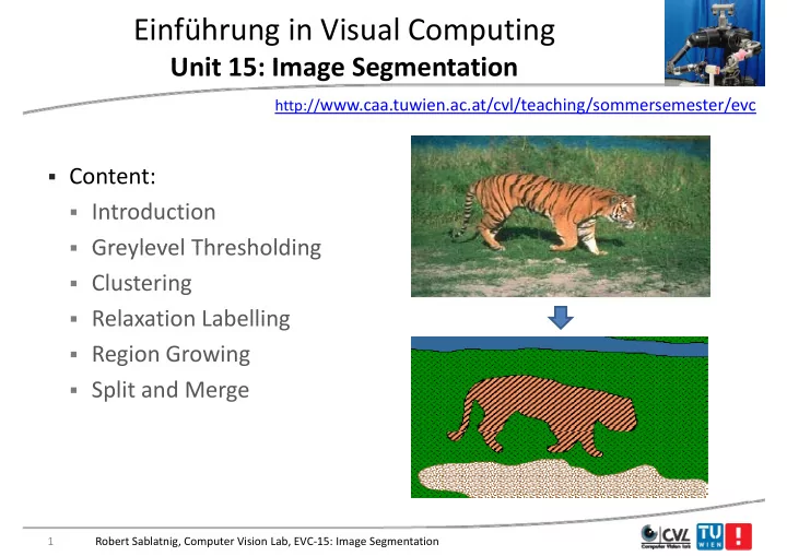
U it 15 I S t ti Unit 15: Image Segmentation

http://www.caa.tuwien.ac.at/cvl/teaching/sommersemester/evc

• Content:
• Introduction
• Greylevel Thresholding
• Greylevel Thresholding
• Clustering
• Relaxation Labelling
• Region Growing
• Split and Merge

1 Robert Sablatnig, Computer Vision Lab, EVC‐15: Image Segmentation

Introduction to Image Segmentation g g

Image Segmentation

Sky Tree Tree ? ? Grass

2 Robert Sablatnig, Computer Vision Lab, EVC‐15: Image Segmentation

Introduction to Image Segmentation g g

The shape shape of an object can be described in terms of:

• Its boundary

boundary – requires image edge detection edge detection

• The region

region it occupies – requires image segmentation image segmentation in homogeneous regions, Image regions generally have g g g g g y homogeneous characteristics (e.g. intensity, texture)

• The purpose

purpose of image segmentation is to partition an image into p p p p g g p g meaningful regions meaningful regions with respect to a particular application

• The segmentation is based on measurements

measurements taken from the The segmentation is based on measurements measurements taken from the image like

• Greylevel Color Texture
• Greylevel, Color, Texture
• Depth
• Motion

3 Robert Sablatnig, Computer Vision Lab, EVC‐15: Image Segmentation

Finding Objects in Images g j g

• To do this we need to divide

the image into two parts g p

• the object of interest (the

foreground foreground) foreground foreground)

• everything else (the

background background)

Sky

background background) Th d fi i i f f d

Tree Tree

• The definition of foreground

and background depends on th t k t h d

Tree ? ?

the task at hand

Grass

4 Robert Sablatnig, Computer Vision Lab, EVC‐15: Image Segmentation

Introduction to Image Segmentation g g

• Usually image segmentation is an initial step

initial step in a series

• f processes aimed at image understanding

image understanding

• f processes aimed at image understanding

image understanding A li ti f i t ti i l d

• Applications of image segmentation include
• Identifying

Identifying objects in a scene for object‐based measurements measurements h i d h such as size and shape

• Identifying objects in a moving scene for object‐based video

compression compression (MPEG4) compression compression (MPEG4)

• Identifying objects which are at different distances from a

sensor using depth measurements depth measurements from a laser range finder sensor using depth measurements depth measurements from a laser range finder enabling path planning path planning for a mobile robot

5 Robert Sablatnig, Computer Vision Lab, EVC‐15: Image Segmentation

Introduction to Image Segmentation g g

• Example 1
• Segmentation based on greyscale

greyscale

• Segmentation based on greyscale

greyscale

• Very simple ‘model’ of greyscale leads to inaccuracies in object

labelling labelling

6 Robert Sablatnig, Computer Vision Lab, EVC‐15: Image Segmentation

Introduction to Image Segmentation g g

• Example 2
• Segmentation based
• Segmentation based
• n texture

texture

• Enables object
• Enables object

surfaces with varying patterns of grey to patterns of grey to be segmented

7 Robert Sablatnig, Computer Vision Lab, EVC‐15: Image Segmentation

Introduction to Image Segmentation g g

• Example 3
• Segmentation based on motion

motion

• Segmentation based on motion

motion

• The main difficulty of motion

segmentation is that an segmentation is that an intermediate step is required to (either implicitly or explicitly) (either implicitly or explicitly) estimate an optical flow field

• The segmentation must be based
• The segmentation must be based
• n this estimate and not, in

general the true flow general, the true flow

8 Robert Sablatnig, Computer Vision Lab, EVC‐15: Image Segmentation

Introduction to Image Segmentation g g

• Example 4
• Segmentation based on depth

depth

• Segmentation based on depth

depth

• This example shows a range

image obtained with a laser

Range image

image, obtained with a laser range finder A segmentation based on the

• A segmentation based on the

range (the object distance from the sensor) is useful in guiding

Segmented image

the sensor) is useful in guiding mobile robots

9 Robert Sablatnig, Computer Vision Lab, EVC‐15: Image Segmentation

Image Segmentation g g

• In analysis of objects in images it is essential to distinguish

between objects of interest

• bjects of interest and "the rest" = background

background.

• Techniques that are used to find objects of interest are referred to

as segmentation segmentation techniques ‐ segmenting the foreground from background.

• Image segmentation describes the division of the image in

homogenous segments homogenous segments (no abrupt intensity changes within segments)

• Edge detection

Edge detection may (not necessarily) produce a segmentation

10 Robert Sablatnig, Computer Vision Lab, EVC‐15: Image Segmentation

What do we mean by “Labeling” an Image? y g g

• When we say we ”extract “ an object in an image , we mean that

we identify the pixels identify the pixels that make it up. y p y p p

• To express this information , we create an array of the same size

as the original image and we give to each pixel each pixel a label label. as the original image and we give to each pixel each pixel a label label.

• All pixels that make up the object
• bject are given the same label

same label . The label is usually a number but it could be anything: a letter or label is usually a number, but it could be anything: a letter, or color.

• Often label images

label images are also referred to as classified images as

• Often label images

label images are also referred to as classified images as they indicate the class class to which each pixel each pixel belongs.

11 Robert Sablatnig, Computer Vision Lab, EVC‐15: Image Segmentation

How can we divide an Image into Uniform Regions ? Regions ?

• Segmentation techniques can be classified as either contextual or

non‐contextual .

• Non‐contextual techniques ignore

ignore the relationships that exist between features features in an image pixels are simply grouped grouped together between features features in an image; pixels are simply grouped grouped together

• n the basis of some global attribute

global attribute, such as grey level.

• Contextual techniques, additionally exploit

exploit the relationships between image features

• features. Thus, a contextual technique might

group together pixels that have similar grey levels and are close to

• ne another .

12 Robert Sablatnig, Computer Vision Lab, EVC‐15: Image Segmentation

Greylevel Threshholding

13

Greylevel Histogram‐based Segmentation y g g

• First, we will look at two very simple non

non‐contextual contextual image segmentation techniques that are based on the greylevel greylevel g q g y g y histogram histogram of an image:

• Thresholding

Thresholding

• Clustering
• We will use a very simple object‐background test image
• We will consider a zero, low and high noise image

Robert Sablatnig, Computer Vision Lab, EVC‐15: Image Segmentation 14

Greylevel Histogram‐based Segmentation y g g

Noise free Low noise High noise

• How do we characterise low noise and high noise?

15 Robert Sablatnig, Computer Vision Lab, EVC‐15: Image Segmentation

Greylevel Histogram‐based Segmentation y g g

Noise free Low noise High noise

• We can consider the histograms of our images

For the noise free image its simply two spikes two spikes at i 100 i 150

• For the noise free image, its simply two spikes

two spikes at i=100, i=150

• For the low noise image, there are two clear peaks

two clear peaks centred on i 100 i 150 i=100, i=150

• For the high noise image, there is a single peak

single peak – two greylevel populations corresponding to object and background have merged

16 Robert Sablatnig, Computer Vision Lab, EVC‐15: Image Segmentation

Greylevel Histogram‐based Segmentation y g g

Low noise Noise free Hi h i

17 Robert Sablatnig, Computer Vision Lab, EVC‐15: Image Segmentation

High noise

Greylevel Histogram‐based Segmentation y g g

• We can define the input image Signal

Signal‐to to‐Noise Noise ratio ratio in terms of the mean mean greylevel greylevel value of the object

• bject pixels and background

background g y g y j p g pixels and the additive noise standard deviation noise standard deviation

S N

b

• /

   

• For our test images :



• S/N (noise free) = 
• S/N (low noise)

= 5

• S/N (high noise) = 2

18 Robert Sablatnig, Computer Vision Lab, EVC‐15: Image Segmentation

Greylevel Thresholding y g

• We can easily understand
• We can easily understand

segmentation based on thresholding by looking at the

Background

thresholding by looking at the histogram histogram of the low noise

• bject/background image
• bject/background image
• There is a clear ‘valley’

clear ‘valley’ between to two peaks two peaks

Object

to two peaks two peaks

• We can define the greylevel

greylevel thresholding thresholding algorithm as follows: thresholding thresholding algorithm as follows:

• If

If the greylevel of pixel p <= <= T th th i l i i bj t bj t i l

T

then then pixel p is is an object

• bject pixel

else else

• Pixel p is a background

background pixel

19 Robert Sablatnig, Computer Vision Lab, EVC‐15: Image Segmentation

Foundation

• If two dominant modes

two dominant modes characterize the image histogram, it is called a bimodal histogram bimodal histogram. Only one threshold

• ne threshold is enough for

g y g partitioning the image.

• If for example an image is composed of two types of light objects
• n a dark background three or more

three or more dominant modes

• n a dark background, three or more

three or more dominant modes characterize the image histogram.

20 Robert Sablatnig, Computer Vision Lab, EVC‐15: Image Segmentation

Foundation (contd.) ( )

• In such a case the histogram has to be partitioned by multiple

multiple thresholds thresholds.

• Multilevel thresholding classifies a point (x y) as belonging
• Multilevel thresholding classifies a point (x,y) as belonging
• to one object class if T1 < f(x,y) <= T2,
• to the other object class if f(x,y) > T2,
• and to the background if f(x,y) <= T1.

21 Robert Sablatnig, Computer Vision Lab, EVC‐15: Image Segmentation

Pixel Classification by Threshold y

• Histogramm
• Problem

Problem: Connected image regions do not always have the g g y same intensity => missing location relation location relation of pixels g p

Original Histogram Segmentation

22 Robert Sablatnig, Computer Vision Lab, EVC‐15: Image Segmentation

Greylevel Thresholding y g

• This simple threshold test begs the obvious question how do we

determine the threshold ?

• Many approaches possible
• Many approaches possible
• Interactive threshold
• Global threshold
• Local threshold
• Minimisation method
• .......

.......

23 Robert Sablatnig, Computer Vision Lab, EVC‐15: Image Segmentation

Global Thresholding

• Basic Global Thresholding:

1

Select an initial estimate initial estimate for T

1.

Select an initial estimate initial estimate for T

2. 2.

Segment Segment the image using T. This will produce two groups two groups of pixels G consisting of all pixels with gray level values >T and

• pixels. G1 consisting of all pixels with gray level values >T and

G2consisting of pixels with values <=T.

3

Comp te the average gray level average gray level al es mean and mean for

3.

Compute the average gray level average gray level values mean1 and mean2 for the pixels in regions G1 and G2. C h h ld h h ld l T ( )

4.

Compute a new threshold new threshold value T=(mean1 +mean2)

5. 5.

Repeat Repeat steps 2 through 4 until difference in T in successive iterations is smaller than smaller than a predefined parameter T0.

24 Robert Sablatnig, Computer Vision Lab, EVC‐15: Image Segmentation

Local Thresholding

• A complex thresholding algorithm is to use a spatially varying

spatially varying

• threshold. This approach is very useful to compensate for the

pp y p effects of non –uniform illumination. If T depends on coordinates x and y, this referred to as Dynamic Dynamic, Adaptive Adaptive or Local Thresholding Local Thresholding. y y p g

• A technique which provides good results is to use edge points

edge points when creating the grey level histogram .

25 Robert Sablatnig, Computer Vision Lab, EVC‐15: Image Segmentation

Local Thresholding ‐ How it Works g

• There are two main approaches to find the threshold:
• the Chow and Kaneko

Chow and Kaneko approach and

• the Chow and Kaneko

Chow and Kaneko approach and

• local thresholding

local thresholding. Th ti b hi d b th th d i th t ll i ll i

• The assumption behind both methods is that smaller image

smaller image regions regions are more likely more likely to have approximately uniform uniform illumination illumination th s being more s itable for thresholding illumination illumination, thus being more suitable for thresholding.

• Chow and Kaneko divide an image into an array of overlapping

bi bi d h fi d h i h h ld i h h ld f h subimages subimages and then find the optimum threshold

• ptimum threshold for each

subimage by investigating its histogram

• histogram. The threshold for each

i l i l i f d b i t l ti th lt f th bi single pixel is found by interpolating the results of the subimages.

26 Robert Sablatnig, Computer Vision Lab, EVC‐15: Image Segmentation

Local Thresholding

• Finding the local threshold is to statistically examine

statistically examine the intensity values of the local neighborhood local neighborhood of each pixel g p

• The statistic

statistic which is most appropriate depends depends largely on

• n the

input image input image. Simple and fast functions include: input image input image. Simple and fast functions include:

1.

The mean mean of the local intensity distribution

mean T

2.

The median median value

mean T 

3.

The mean of the minimum minimum and maximum maximum values,

median T 

2 max min  T

Robert Sablatnig, Computer Vision Lab, EVC‐15: Image Segmentation 27

2

Local Thresholding Example g p

Image contains a strong illumination gradient, global global thresholding thresholding produces a very poor result Source Image

28 Robert Sablatnig, Computer Vision Lab, EVC‐15: Image Segmentation

Local Thresholding

• Improve: If threshold employed is not

the mean, but (mean‐C), where C is a , ( ), constant

• Using this statistic, all pixels which exist

in a uniform neighborhood (e g along in a uniform neighborhood (e.g. along the margins) are set to background

The result for a 7×7 The result for a 7×7 neighborhood and C=7

29 Robert Sablatnig, Computer Vision Lab, EVC‐15: Image Segmentation

Pixel Classification by Threshold y

• Interactive, imprecise threshold

=> Threshold influences segmentation => Threshold influences segmentation

30 Robert Sablatnig, Computer Vision Lab, EVC‐15: Image Segmentation

Thresholding Example g p

• Let‘s take a 7x7 image

3 5 7 3 4 2 1 2 4 9 10 22 9 3 3 5 12 11 15 10 3 3 5 12 11 15 10 3 5 6 11 9 17 19 1 2 3 11 12 18 16 2 3 6 8 10 18 9 5 3 6 8 10 18 9 5 4 6 7 8 3 3 1 Robert Sablatnig, Computer Vision Lab, EVC‐15: Image Segmentation 31

Thresholding Example g p

• And a threshold T= 7 (mean)

3 5 7 3 4 2 1 2 4 9 10 22 9 3 3 5 12 11 15 10 3 3 5 12 11 15 10 3 5 6 11 9 17 19 1 2 3 11 12 18 16 2 3 6 8 10 18 9 5 3 6 8 10 18 9 5 4 6 7 8 3 3 1 Robert Sablatnig, Computer Vision Lab, EVC‐15: Image Segmentation 32

Thresholding Example g p

• Alternatively T= 6 (Median)

3 5 7 3 4 2 1 2 4 9 10 22 9 3 3 5 12 11 15 10 3 3 5 12 11 15 10 3 5 6 11 9 17 19 1 2 3 11 12 18 16 2 3 6 8 10 18 9 5 3 6 8 10 18 9 5 4 6 7 8 3 3 1 Robert Sablatnig, Computer Vision Lab, EVC‐15: Image Segmentation 33

Thresholding Example g p

• Alternatively T= 12 ((min+max)/2)

3 5 7 3 4 2 1 2 4 9 10 22 9 3 3 5 12 11 15 10 3 3 5 12 11 15 10 3 5 6 11 9 17 19 1 2 3 11 12 18 16 2 3 6 8 10 18 9 5 3 6 8 10 18 9 5 4 6 7 8 3 3 1 Robert Sablatnig, Computer Vision Lab, EVC‐15: Image Segmentation 34

Thresholding Example g p

• Or T= 10

3 5 7 3 4 2 1 2 4 9 10 22 9 3 3 5 12 11 15 10 3 3 5 12 11 15 10 3 5 6 11 9 17 19 1 2 3 11 12 18 16 2 3 6 8 10 18 9 5 3 6 8 10 18 9 5 4 6 7 8 3 3 1 Robert Sablatnig, Computer Vision Lab, EVC‐15: Image Segmentation 35

Clustering

36

Greylevel Clustering y g

• Consider an idealized object/background histogram

Background Object

c1 c2

• Clustering tries to separate the histogram into 2 groups defined by

two cluster centres c1 and c2 two cluster centres c1 and c2

37 Robert Sablatnig, Computer Vision Lab, EVC‐15: Image Segmentation

Greylevel Clustering y g

• A nearest neighbour

nearest neighbour clustering algorithm allows us perform a greylevel segmentation using clustering

• A simple case of a more general and widely used K‐means

means clustering

• A simple iterative algorithm which has known convergence

properties

• Given a set of greylevels:

 

g g g N ( ), ( )...... ( ) 1 2

• We can partition this set into two groups

and

 

g g g N

1 1 1 1

1 2 ( ), ( )...... ( )

 

g g g N

2 2 2 2

1 2 ( ), ( )...... ( )

38 Robert Sablatnig, Computer Vision Lab, EVC‐15: Image Segmentation

Greylevel Clustering y g

• Compute the local means of each group

N

1

1

2

1

N

and R d fi th i

c N g i

i 1 1 1 1

1  



( )







2

1 2 2 2

) ( 1

i

i g N c

• Re‐define the new groupings:

g k c g k c k N 1 ( ) ( )     g k c g k c k N

1 1 1 2 1

1 ( ) ( ) ..   g k c g k c k N

2 2 2 1 2

1 ( ) ( )    

• In other words all grey levels

all grey levels in Set 1 are nearer to cluster center nearer to cluster center

g k c g k c k N

2 2 2 1 2

1 ( ) ( ) .. 

• In other words all grey levels

all grey levels in Set 1 are nearer to cluster center nearer to cluster center c1 and all grey levels in Set 2 are nearer to cluster center c2

39 Robert Sablatnig, Computer Vision Lab, EVC‐15: Image Segmentation

Greylevel Clustering y g

• But, we have a chicken and egg

chicken and egg situation

• The problem with the above definition
• The problem with the above definition

is that each group mean is defined in terms of the partitions and vice versa terms of the partitions and vice versa The sol tion is to define an iterati e

• The solution is to define an iterative

algorithm and worry about the convergence of the algorithm later convergence of the algorithm later

40 Robert Sablatnig, Computer Vision Lab, EVC‐15: Image Segmentation

Greylevel Clustering y g

• The iterative algorithm is as follows

Initialize the label of each pixel randomly randomly Initialize the label of each pixel randomly randomly Repeat Repeat Repeat Repeat c1= mean of pixels assigned to object label f i l i d b k d l b l c2= mean of pixels assigned to background label C i i

 

Compute partition Compute partition

 

g g g N

1 1 1 1

1 2 ( ), ( )...... ( )

 

g g g N

2 2 2 2

1 2 ( ), ( )...... ( )

Until none none pixel labelling labelling changes changes

 

41 Robert Sablatnig, Computer Vision Lab, EVC‐15: Image Segmentation

Greylevel Clustering y g

• Two questions to answer
• Does this algorithm converge

converge?

• Does this algorithm converge

converge?

• If so, to what

to what does it converge?

• We can show that the algorithm is guaranteed to converge and

also that it converges to a sensible result

42 Robert Sablatnig, Computer Vision Lab, EVC‐15: Image Segmentation

Greylevel Clustering y g

g2 g1

c c c1 c2

43 Robert Sablatnig, Computer Vision Lab, EVC‐15: Image Segmentation

Greylevel Clustering y g

• Clustering
• Finds groups of pixels with
• Finds groups of pixels with

similar properties similar properties

• Does not guarantee

not guarantee that these

• Does not guarantee

not guarantee that these groups form continuous areas continuous areas in the image in the image

• Even if it does, edges

edges of these areas tend to be uneven uneven areas tend to be uneven uneven

44 Robert Sablatnig, Computer Vision Lab, EVC‐15: Image Segmentation

Relaxation Labelling

45

Relaxation Labelling

• All of segmentation algorithms considered so far are based on

histogram of the image g g

• This ignores

ignores the greylevels of each pixels’ neighbours neighbours which will strongly influence strongly influence the classification classification of each pixel strongly influence strongly influence the classification classification of each pixel

• Objects are usually represented by a spatially contiguous

spatially contiguous set of pixels pixels

• Trivial example of a likely pixel miss‐classification:

Object k d

46

Background

Robert Sablatnig, Computer Vision Lab, EVC‐15: Image Segmentation

Relaxation Labelling: Probabilities g

• Relaxation labelling

Relaxation labelling is a general technique in computer vision which is able to incorporate constraints constraints (such as spatial p ( p continuity) into image labelling problems

• Assume a simple object/background image

Assume a simple object/background image

• p(i) is the probability that pixel i is a background pixel

(1 p(i)) is the probabilit that pi el i is a object pi el

• (1‐ p(i)) is the probability that pixel i is a object pixel
• Define the 8‐neighbourhood of pixel i as {i1,i2,….i8}

i1 i2 i3 i i4 i5

47

i6 i7 i8

Robert Sablatnig, Computer Vision Lab, EVC‐15: Image Segmentation

Relaxation Labelling: Consistencies g

Define consistencies consistencies c and c

• Define consistencies

consistencies cp and cn

• Positive cp and negative cn encourages neighbouring pixels to

h h l b l have the same label

• Setting these consistencies to appropriate values will encourage

spatially contiguous object and background regions

• We assume again a bi‐modal object/background histogram with

maximum greylevel gmax

Background Object j

48

gmax

Robert Sablatnig, Computer Vision Lab, EVC‐15: Image Segmentation

Relaxation Labelling: Algorithm g g

• We can initialize the probabilities

i i

( )( )

( ) /

• Our relaxation algorithm must ‘drive’ the background pixel

background pixel

p i g i g

( ) max

( ) ( ) / 

Our relaxation algorithm must drive the background pixel background pixel probabilities p(i) to 1 and the object pixel

• bject pixel probabilities to 0
• We want to take into account:
• We want to take into account:
• Neighbouring probabilities

Neighbouring probabilities p(i1), p(i2), …… p(i8) Th i l i l d

• The consistency values

consistency values cp and cn

• We would like our algorithm to ‘saturate

saturate’ such that p(i)~1

• We can then convert the probabilities to labels by multiplying

by 255

49 Robert Sablatnig, Computer Vision Lab, EVC‐15: Image Segmentation

Relaxation Labelling: Algorithm g g

• We can derive the equation for relaxation labelling by first

considering a neighbour i1 of pixel i g g

1

p

• We would like to evaluate the contribution

contribution to to the increment increment in p(i) from i1 p(i) from i1

• Let this increment be q(i1)

We can e al ate q(i ) b taking into acco nt the consistencies We can evaluate q(i1) by taking into account the consistencies

• We can apply a simple decision rule to determine the contribution

to the increment q(i1) from pixel i1

• If p(ii) >0.5

>0.5 the contribution from pixel i1 increments increments p(i)

• If p(ii) <0.5 the contribution from pixel i1 decrements

decrements p(i) p( i) p

1

p( )

50 Robert Sablatnig, Computer Vision Lab, EVC‐15: Image Segmentation

Relaxation Labelling: Algorithm g g

• Since cp >0 and cn <0 its easy to see that the following expression

for q(i1) has the right properties We can now average all average all the contributions from the 8 neighbours neighbours

)) ( 1 ( ) ( ) (

1 1 1

i p c i p c i q

n p

  

• We can now average all

average all the contributions from the 8‐neighbours neighbours

• f i to get the total increment to p(i)

1

8

E t h k th t 1< (i)<1 f 1< <1

) )) ( 1 ( ) ( ( 8 1 ) (

1





   

h h n h p

i p c i p c i p

• Easy to check that –1<p(i)<1 for ‐1< cp ,cn <1
• Can update p(i) as follows:

p i p i p i

r r ( ) ( )

( ) ( )( ( ))





1

1 

• Ensures that p(i) remains positive

p i p i p i

( ) ( )

( ) ~ ( )( ( ))  1 

• Basic form of the relaxation equation

51 Robert Sablatnig, Computer Vision Lab, EVC‐15: Image Segmentation

Relaxation Labelling: Normalization g

• We need to normalize

normalize the probabilities p(i) as they must stay in the range {0..1} g { }

• After every iteration p(r)(i) is rescaled

rescaled to bring it back into the correct range correct range

• Remember our requirement that likely background pixel

probabilities are ‘driven’ to 1 probabilities are driven to 1

• One possible approach is to use a constant normalisation

constant normalisation factor

( ) ( ) ( )

p i p i p i

r r i r ( ) ( ) ( )

( ) ( ) / max ( ) 

0 9 0 9 0 9 0.9 0.9 0.9

• the central background pixel probability

may get stuck at 0.9 if max(p(i))=1

0.9 0.9 0.9 0.9 0.9 0.9

52 Robert Sablatnig, Computer Vision Lab, EVC‐15: Image Segmentation

Relaxation Labelling: Normalization g

• The following normalisation equation has all the right properties
• It can be derived from the general theory of relaxation labelling
• It can be derived from the general theory of relaxation labelling

p i p i p i

r r ( ) ( ) ( ) ( )

( ) ( )( ( ))  

1 1 1

1 

• We can check to see if this normalisation equation has the correct

p i p i p i p i p i

r r ( ) ( )

( ) ( )( ( )) ( ( ))( ( ))    

  1 1

1 1 1  

• We can check to see if this normalisation equation has the correct

‘saturation’ properties

• When p(r‐1)(i)=1 p(r)(i)=1
• When p

(i)=1, p (i)=1

• When p(r‐1)(i)=0, p(r)(i)=0
• When p(r‐1)(i)=0 9 and p(i)=0 9 p(r)(i)=0 994
• When p(r 1)(i)=0.9 and p(i)=0.9, p(r)(i)=0.994
• When p(r‐1)(i)=0.1 and p(i)=‐0.9, p(r)(i)=0.012

W th t (i) t 0 1

• We can see that p(i) converges to 0 or 1

53 Robert Sablatnig, Computer Vision Lab, EVC‐15: Image Segmentation

Relaxation Labelling: Results g

• Algorithm performance on the high noise image
• Comparison with thresholding
• Comparison with thresholding

High noise circle image ’ Optimum’ threshold Relaxation labeling 20 iterations

54 Robert Sablatnig, Computer Vision Lab, EVC‐15: Image Segmentation

Relaxation Labelling: Results g

• The following is an example of a case where the algorithm has

problems due to the thin structure in the clamp image p p g

l i l i d l i clamp image

• riginal

clamp image noise added segmented clamp image 10 iterations

55 Robert Sablatnig, Computer Vision Lab, EVC‐15: Image Segmentation

Relaxation Labelling: Results g

• Applying the algorithm to normal greylevel images we can see a

clear separation into light and dark areas p g

Original 2 iterations 5 iterations 10 iterations

56 Robert Sablatnig, Computer Vision Lab, EVC‐15: Image Segmentation

Relaxation Labelling: Results g

• The histogram of each image shows the clear saturation to 0 and

255

h(i)

5000.00

h(i)

3000.00 4000.00 Original 2000.00 Original 2 iterations 5 iterations 10 iterations 1000.00 0.00 0.00 50.00 100.00 150.00 200.00 250.00

i

57 Robert Sablatnig, Computer Vision Lab, EVC‐15: Image Segmentation

Region Growing

58

Region‐Based Segmentation g g

• We want smooth regions

smooth regions in the image

• Region growing
• Start with a small ‘seed’

small ‘seed’

in the image

• We still want the pixels in

each region to be similar similar

• Start with a small seed

small seed and expand by adding similar pixels each region to be similar similar, and those in adjacent regions to be different different similar pixels

• Split and merge

regions to be different different

• One way to do this is to

work with regions regions rather

• Splitting divides

divides regions that are inconsistent inconsistent work with regions regions rather than pixels

• Merging combines

combines adjacent regions that are consistent consistent

59 Robert Sablatnig, Computer Vision Lab, EVC‐15: Image Segmentation

Region Growing g g

• Simple approach: start from some pixels (seeds

seeds) representing distinct image regions and to grow grow them, until they cover the g g g , y entire entire image image

• For region growing we need a rule describing a growth

growth mechanism mechanism and a rule checking the homogeneity checking the homogeneity of the regions mechanism mechanism and a rule checking the homogeneity checking the homogeneity of the regions after each growth step

• Growth mechanism

Growth mechanism: at each stage k and for each region R (k)

• Growth mechanism

Growth mechanism: at each stage k and for each region Ri(k), i = 1,…,N, check if there are unclassified pixels unclassified pixels in the 8‐neigh‐ b h d f h i l f th i b d bourhood of each pixel of the region border

• Before assigning such a pixel x to a region Ri(k),we check if the

i h i i h i ( (k) { }) lid lid region homogeneity region homogeneity: P(Ri(k) U {x}) = TRUE , is valid valid

60 Robert Sablatnig, Computer Vision Lab, EVC‐15: Image Segmentation

Growth Mechanism

• The arithmetic mean m and standard deviation sd of a class Ri

having n pixels: having n pixels:





n

y x I m ) , ( 1



 

n

m y x I sd

2

] ) ( [ 1

• can be used to decide if the merging of the two regions R R is



 i

y n

1

) , (







i

m y x I n sd

1

] ) , ( [

• can be used to decide if the merging of the two regions R1,R2 is

allowed

• if

two regions are merged

2 1 ) (     i i sd k m m

• if

two regions are merged

2 , 1 ), (

2 1

    i i sd k m m

61 Robert Sablatnig, Computer Vision Lab, EVC‐15: Image Segmentation

Region Homogeneity g g y

• Homogeneity test: if the pixel intensity is close to the region

mean value

i i

T m y x I m    ) , (

• Threshold Ti varies depending on the region Rn and the intensity
• f the pixel I(x,y) and can be chosen by:
• e p e ( ,y) a d ca be c ose by

T i m i sd Ti           ) ( ) ( 1 i m     ) (

62 Robert Sablatnig, Computer Vision Lab, EVC‐15: Image Segmentation

Region Growing Summary g g y

• Region growing starts with a small patch of seed

small patch of seed pixels

• Compute statistics about the region
• Compute statistics about the region
• Check neighbors to see if they can be added

h

• Re‐compute the statistics
• This procedure repeats until the region stops growing
• Simple example: We compute the mean grey level of the pixels

Simple example: We compute the mean grey level of the pixels in the region

• Neighbors are added if their grey level is near the average
• Neighbors are added if their grey level is near the average

63 Robert Sablatnig, Computer Vision Lab, EVC‐15: Image Segmentation

Region Growing Example g g p

3 5 7 3 4 2 1 2 4 9 10 22 9 3 3 5 12 11 15 10 3 3 5 12 11 15 10 3 5 6 11 9 17 19 1 2 3 11 12 18 16 2 3 6 8 10 18 9 5 3 6 8 10 18 9 5 4 6 7 8 3 3 1 64 Robert Sablatnig, Computer Vision Lab, EVC‐15: Image Segmentation

Region Growing Example g g p

• We start with T=10

3 5 7 3 4 2 1 2 4 9 10 22 9 3 3 5 12 11 15 10 3 3 5 12 11 15 10 3 5 6 11 9 17 19 1 2 3 11 12 18 16 2 3 6 8 10 18 9 5 3 6 8 10 18 9 5 4 6 7 8 3 3 1 Robert Sablatnig, Computer Vision Lab, EVC‐15: Image Segmentation 65

Region Growing Example g g p

• Check neighbors in line 4 (11,17,19) in 8‐neighborhood

3 5 7 3 4 2 1 2 4 9 10 22 9 3 3 5 12 11 15 10 3 3 5 12 11 15 10 3 5 6 11 9 17 19 1 2 3 11 12 18 16 2 3 6 8 10 18 9 5 3 6 8 10 18 9 5 4 6 7 8 3 3 1 Robert Sablatnig, Computer Vision Lab, EVC‐15: Image Segmentation 66

Region Growing Example g g p

• Check neighbors in line 5 (11,12,18,16) in 8‐neighborhood

3 5 7 3 4 2 1 2 4 9 10 22 9 3 3 5 12 11 15 10 3 3 5 12 11 15 10 3 5 6 11 9 17 19 1 2 3 11 12 18 16 2 3 6 8 10 18 9 5 3 6 8 10 18 9 5 4 6 7 8 3 3 1 Robert Sablatnig, Computer Vision Lab, EVC‐15: Image Segmentation 67

Region Growing Example g g p

• Check neighbors in line 3 (12,11,15,10) in 8‐neighborhood

3 5 7 3 4 2 1 2 4 9 10 22 9 3 3 5 12 11 15 10 3 3 5 12 11 15 10 3 5 6 11 9 17 19 1 2 3 11 12 18 16 2 3 6 8 10 18 9 5 3 6 8 10 18 9 5 4 6 7 8 3 3 1 Robert Sablatnig, Computer Vision Lab, EVC‐15: Image Segmentation 68

Region Growing Example g g p

69 Robert Sablatnig, Computer Vision Lab, EVC‐15: Image Segmentation

Split and Merge

70

Split and Merge p g

• The opposite approach to region growing is region shrinking

(Splitting Splitting) ( p g p g)

• It is a top

top‐down down approach and it starts with the assumption that the entire image is homogeneous homogeneous the entire image is homogeneous homogeneous

• If this is not true, the image is split into four sub images

four sub images This splitting proced re is repeated recursively recursively ntil e split the

• This splitting procedure is repeated recursively

recursively until we split the image into homogeneous regions homogeneous regions

71 Robert Sablatnig, Computer Vision Lab, EVC‐15: Image Segmentation

Split p

• If the original image is square N x N, having dimensions that are

powers of 2(N = 2n): p ( )

• All regions produced but the splitting algorithm are squares

having dimensions M x M , where M is a power of 2 as well having dimensions M x M , where M is a power of 2 as well (M=2m,M<= n).

• Since the procedure is recursive it produces an image
• Since the procedure is recursive, it produces an image

representation that can be described by a tree whose nodes have four sons each four sons each

• Such a tree is called a Quadtree

Quadtree.

72 Robert Sablatnig, Computer Vision Lab, EVC‐15: Image Segmentation

Quadtrees

73 Robert Sablatnig, Computer Vision Lab, EVC‐15: Image Segmentation

Split Example p p

• Splits original image into 4 sub‐images

74 Robert Sablatnig, Computer Vision Lab, EVC‐15: Image Segmentation

Split Example p p

• 3 sub‐images are

homogeneous homogeneous

• Upper right sub‐image

hast to be split

75 Robert Sablatnig, Computer Vision Lab, EVC‐15: Image Segmentation

Split Example p p

• 3 sub‐sub‐images are

homogeneous homogeneous

• Lower right sub‐sub‐

image hast to be split

76 Robert Sablatnig, Computer Vision Lab, EVC‐15: Image Segmentation

Split Example p p

77 Robert Sablatnig, Computer Vision Lab, EVC‐15: Image Segmentation

Split and Merge p g

• Splitting disadvantage

disadvantage: creates regions that may be adjacent and homogeneous, but not not merged merged g , g

• Split and Merge method: iterative algorithm that includes both

splitting and merging at each each iteration iteration: splitting and merging at each each iteration iteration:

• (P(R)= False): if a region R is inhomogeneous then split into four

sub regions sub regions

• (P(Ri U Rj) = TRUE): if two adjacent regions Ri,Rj are

homogeneous they are merged homogeneous, they are merged

• The algorithm stops when no further splitting or merging is

ibl possible

• Split and Merge algorithm produces more compact regions

more compact regions than h l l h the pure splitting algorithm

78 Robert Sablatnig, Computer Vision Lab, EVC‐15: Image Segmentation

Applications pp

• 3D – Imaging : A basic task in 3‐D image processing is

segmentation of images which classifies voxels/pixels into objects g g /p j

• r groups.
• 3‐D image segmentation makes it possible to create 3‐D rendering

3 D image segmentation makes it possible to create 3 D rendering for multiple objects and performs quantitative analysis for size, density or other parameters of detected objects. de s y o o e pa a e e s o de ec ed objec s

• Several applications in the field of Medicine like magnetic

resonance imaging (MRI) resonance imaging (MRI).

79 Robert Sablatnig, Computer Vision Lab, EVC‐15: Image Segmentation

Results – Region Growing g g

80 Robert Sablatnig, Computer Vision Lab, EVC‐15: Image Segmentation

Results – Region Split g p

81 Robert Sablatnig, Computer Vision Lab, EVC‐15: Image Segmentation

Results – Region Split and Merge g p g

82 Robert Sablatnig, Computer Vision Lab, EVC‐15: Image Segmentation

Results – Region Growing g g

83 Robert Sablatnig, Computer Vision Lab, EVC‐15: Image Segmentation

Results – Region Split g p

84 Robert Sablatnig, Computer Vision Lab, EVC‐15: Image Segmentation

Results – Region Split and Merge g p g

Robert Sablatnig, Computer Vision Lab, EVC‐15: Image Segmentation 85