Einfhrung in Visual Computing U it 11 P i t O Unit 11: Point - - PowerPoint PPT Presentation

Einführung in Visual Computing

U it 11 P i t O ti Unit 11: Point Operations

http://www.caa.tuwien.ac.at/cvl/teaching/sommersemester/evc

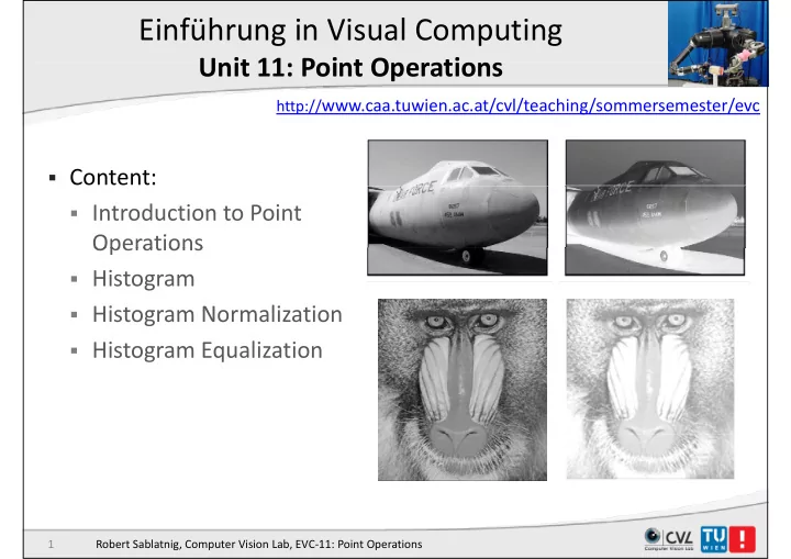
• Content:
• Introduction to Point

Operations Operations

• Histogram

Histogram Normali ation

• Histogram Normalization
• Histogram Equalization

1 Robert Sablatnig, Computer Vision Lab, EVC‐11: Point Operations

Point Operations p

mainly applied in the pre‐processing step:

• Intensity of a new pixel is dependent on the original pixel only:
• Intensity of a new pixel is dependent on the original pixel only:
• Example: Inversion, Threshold, Brightness Enhancement,

Contrast Enhancement Contrast Enhancement…

2 Robert Sablatnig, Computer Vision Lab, EVC‐11: Point Operations

Point Operations p

• Point Operations perform a mapping of the pixel values without

changing the size, geometry, or local structure of the image g g , g y, g

• Each new pixel value I’(u,v) depends on the previous value I(u,v)

at the same position and on a mapping function f() at the same position and on a mapping function f()

• The function f() is independent of the coordinates

S ch operation is called “homogeneo s”

• Such operation is called “homogeneous”

3 Robert Sablatnig, Computer Vision Lab, EVC‐11: Point Operations

Point Operations p

4 Robert Sablatnig, Computer Vision Lab, EVC‐11: Point Operations

Point Operations p

Example of homogeneous point operations:

• Modifying image brightness or contrast
• Modifying image brightness or contrast
• Applying arbitrary intensity transformation (curves)

Q ti i ( t i i ) i

• Quantizing (posterizing) images
• Global thresholding
• Gamma correction
• Color transformations

5 Robert Sablatnig, Computer Vision Lab, EVC‐11: Point Operations

Definition of Point Operations p

• New intensity value (gray‐level) of a

pixel only depends on the previous l value.

• Transformation is performed on the

pixel intensity value using a pixel intensity value using a mapping function:

• linear or
• non‐linear.
• Mapping is usually implemented

pp g y p with look‐up tables (LUT).

• Following functions are possible:
• Linear
• stepwise linear

I‘(u,v) ← a · I (u,v) + b

• non‐linear

6 Robert Sablatnig, Computer Vision Lab, EVC‐11: Point Operations

Point Operations: Identity Function p y

• The identity function does not alter

any pixel values.

Before: I‘(u,v) ← a · I (u,v) + b

y p

After:

7 Robert Sablatnig, Computer Vision Lab, EVC‐11: Point Operations

a = 1, b = 0

Point Operations: Inversion Function p

• Inversion means that dark become

bright and vice versa.

Before:

g

I‘(u,v) ← a · I (u,v) + b After:

8 Robert Sablatnig, Computer Vision Lab, EVC‐11: Point Operations

a = ‐1, b = q = 255

Example: Inversion Transformation p

Fi i f lid G l / W d DIP b k b i (Ch 3) Figure is from slides at Gonzalez/ Woods DIP book website (Chapter 3)

Inversion Transformation

• Inverting Images

I‘(u,v) ← −I(u,v) + q = q − I(u, v).

Threshold Operation p

• Thresholding an image is a special type of quantization that

separates the pixel values in two classes, depending on a given p p , p g g threshold value pth

• The threshold function maps all the pixels to one of two fixed

The threshold function maps all the pixels to one of two fixed intensity values po, p1 0 < pth ≤ pmax

• Example: binarization: po=0, p1=1

11 Robert Sablatnig, Computer Vision Lab, EVC‐11: Point Operations

Threshold Operation p

pth p1 p0

12 Robert Sablatnig, Computer Vision Lab, EVC‐11: Point Operations

Histograms

Point Operations: Threshold Function p

Before:

• Thresholding means a reduction

to only two different color levels

Before:

y upon a certain threshold value.

After:

13 Robert Sablatnig, Computer Vision Lab, EVC‐11: Point Operations

Point Operations: Gray Level Reduction F nction Function

Before:

• Gray‐level reduction reduces the

number of intensity levels (e.g. 4

Before:

y ( g different levels).

After:

14 Robert Sablatnig, Computer Vision Lab, EVC‐11: Point Operations

Point Operations: Brightness Increasing F nction Function

Before: Before:

• Generally the intensity values are
• increased. Note: Clipping may occur.

Before: Before:

pp g y

I‘(u,v) ← a · I (u,v) + b After: After:

15 Robert Sablatnig, Computer Vision Lab, EVC‐11: Point Operations

a = 1, b = 90

Point Operations: Brightness Reducing F nction Function

Before:

• Generally the intensity values are

reduced

Before: I‘(u,v) ← a · I (u,v) + b After:

16 Robert Sablatnig, Computer Vision Lab, EVC‐11: Point Operations

a = 1, b = ‐90

Point Operations: Contrast Enhancing F nction Function

Before:

• Intensity value that formerly were close

together are now further apart

Before:

(spreading). Note: Clipping may occur.

I‘(u,v) ← a · I (u,v) + b After:

17 Robert Sablatnig, Computer Vision Lab, EVC‐11: Point Operations

a = 0,01, b = 1

Point Operations: Contrast Reducing Function p g

Before:

• Intensity value that formerly were wider apart

are now closer (narrowing). The resulting

Before:

( g) g image does not contain the full intensity range.

I‘(u,v) ← a · I (u,v) + b After:

18 Robert Sablatnig, Computer Vision Lab, EVC‐11: Point Operations

a = 90, b = 1

Point Operations: Gamma Correcting F nction Function

Before:

• Example of a non‐linear mapping

function.

Before: After:

19 Robert Sablatnig, Computer Vision Lab, EVC‐11: Point Operations

Photoshop: Image ‐ Adjustments ‐ Curves p g j

Robert Sablatnig, Computer Vision Lab, EVC‐11: Point Operations 20

Histogram

Histogram g

• The histogram function is defined over all possible intensity levels.
• For each intensity level its value is equal to the number of the
• For each intensity level, its value is equal to the number of the

pixels with that intensity.

• Consider a 5x5 image with integer intensities in the range
• Consider a 5x5 image with integer intensities in the range

between one and eight: 1 8 4 3 4 1 1 1 7 8 1 1 1 7 8 8 8 3 3 1 2 2 1 5 2 2 2 1 5 2 1 1 8 5 2

22 Robert Sablatnig, Computer Vision Lab, EVC‐11: Point Operations

Example p

1 8 4 3 4 1 1 1 7 8 8 8 3 3 1 2 2 1 5 2 1 1 8 5 2 1 2 3 4 5 6 7 8

23 Robert Sablatnig, Computer Vision Lab, EVC‐11: Point Operations

Histogram Function g

H(x) = card{(u,v) | I(u,v)=k}, k {0,...,q}

1

n

2

n

3

n

4

n

5

n

6

n

7

n

8

n

f ) (

k k

n r f  ) (

1 2 3 4 5 6 7 8 1 2 3 4 5 6 7 8

Histogram Function g

8 ) (  r f 4 ) ( 8 ) (

2 1

  r f r f

1

n

2

n

3

n

4

n

5

n

6

n

7

n

8

n

3 ) ( 3 ) (

4 3

  r f r f ) ( 2 ) ( ) (

5 4

 f r f f 1 ) ( ) (

7 6

  r f r f

1 2 3 4 5 6 7 8

5 ) ( 8  r f

1 2 3 4 5 6 7 8

Histogram g

• Assume that the digital image has q discrete gray levels and that

nk, k = 0, ..., q‐1, is the number of pixel having intensity k. The histogram is given by:

n r h r p

k k k

  ) ( ) (

where p is the normalized histogram function, n the total number

n n

• f image pixels. nk are the number of pixels in the bin assigned to

pixels with intensity level k.

• It gives a measure of how likely is for a pixel to have a certain
• intensity. That is, it gives the probability of occurrence the

intensity intensity.

• The sum of the normalized histogram function over the range of

all intensities is 1 all intensities is 1.

Robert Sablatnig, Computer Vision Lab, EVC‐11: Point Operations 26

Histogram g

• The histogram function can be plotted
• graphically. The image histogram carries

g p y g g important information about the image content.

Robert Sablatnig, Computer Vision Lab, EVC‐11: Point Operations 27

Histogram g

• Distribution of gray‐levels can be judged by

measuring a histogram: g g

• For B‐bit image, initialize q=2B counters with 0
• Loop over all pixels x y
• Loop over all pixels x,y
• When encountering gray level f(rk)=i,

increment co nter r increment counter rk

• Histogram can be interpreted as an estimate of

h b bili d i f i ( df) f h the probability density function (pdf) of the underlying random process.

• You can also use fewer, larger bins to trade off

amplitude resolution against sample size.

28 Robert Sablatnig, Computer Vision Lab, EVC‐11: Point Operations

Histogram g

• Histogram on the right corresponds to the image on the left. It is a

statistical measure of the occurrence of different color levels.

29 Robert Sablatnig, Computer Vision Lab, EVC‐11: Point Operations

Histogram g

R h l i f f f h i

• Represents the relative frequency of occurrence of the various gray

levels in the image

• For each gray level count the # of pixels having that level
• For each gray level, count the # of pixels having that level
• Can group nearby levels to form a big bin & count #pixels in it

( From Matlab Image Toolbox Guide Fig.10‐4 )

30 Robert Sablatnig, Computer Vision Lab, EVC‐11: Point Operations

Histogram (cont’d) g ( )

• Interpretation
• Treat pixel values as random variables

p

• Histogram is an estimate of the probability distribution
• “Unbalanced” histogram does not fully utilize the dynamic range

Unbalanced histogram does not fully utilize the dynamic range

• Low contrast image ~ histogram concentrating in a narrow

luminance range u a ce a ge

• Under‐exposed image ~ histogram concentrating on the dark

side

• Over‐exposed image ~ histogram concentrating on the bright

side

• Balanced histogram gives more pleasant look and reveals rich

content

31 Robert Sablatnig, Computer Vision Lab, EVC‐11: Point Operations

Example: Balanced and Unbalanced Histograms Histograms

Figure is from slides at Gonzalez/ Woods DIP book website (Chapter 3) 32 Robert Sablatnig, Computer Vision Lab, EVC‐11: Point Operations

Histogram and Point Operation g p

• Relationship Histogramm – Position in image
• Anges in histogramm will change image content irreversively
• Anges in histogramm will change image content irreversively

Robert Sablatnig, Computer Vision Lab, EVC‐11: Point Operations 33

Histogram g

• If pixel values are concentrated in the low image densities the

image appears dark.

• If the intensity values are not spread entirely over the possible

intensity interval the image is said to be of low contrast.

34 Robert Sablatnig, Computer Vision Lab, EVC‐11: Point Operations

Histogram g

• If the intensity values are spread entirely over the possible

intensity interval the image is said to be rich of contrast. y g

35 Robert Sablatnig, Computer Vision Lab, EVC‐11: Point Operations

Histogram g

• If the image histogram is concentrated on a small intensity region,

the image contrast is poor and the subjective image quality is low. g p j g q y

• Image quality can be enhanced by modifying its histogram This
• Image quality can be enhanced by modifying its histogram. This

can be done in two ways: Histogram Normali ation (Stretching)

• Histogram Normalization (Stretching)
• Histogram Equalization

36 Robert Sablatnig, Computer Vision Lab, EVC‐11: Point Operations

Color Histogram g

• Histograms can be computed

for each channel of a color image.

• The luminance channel the

average of red, green and blue in this case.

37 Robert Sablatnig, Computer Vision Lab, EVC‐11: Point Operations

Photoshop: Image ‐ Adjustments ‐ Levels p g j

Robert Sablatnig, Computer Vision Lab, EVC‐11: Point Operations 38

Histogram Normalization

Histogram Normalization g

40 Robert Sablatnig, Computer Vision Lab, EVC‐11: Point Operations

Histogram Normalization g

• Goal: utilization of the

complete gray level range p g y g

• => linear spreading of gray
• => linear spreading of gray

levels to the complete gray level range

• riginal

level range ) ( I

min max min

) , ( ) , ( ' q q q v u I q v u I    

stretched

41 Robert Sablatnig, Computer Vision Lab, EVC‐11: Point Operations

Contrast Stretching: Example g p

h d

• riginal

stretched

42 Robert Sablatnig, Computer Vision Lab, EVC‐11: Point Operations

Contrast Stretching for Low‐Contrast Images g g

• Stretch the over‐concentrated graylevels in histogram via a

nonlinear mapping pp g

• Piece‐wise linear stretching function

) ( q v u I

min min max min min max

) , ( ) ( ) , ( ' p q q q v u I p p v u I      

43 Robert Sablatnig, Computer Vision Lab, EVC‐11: Point Operations

Photoshop: Image ‐ Adjustments ‐ Levels p g j

Robert Sablatnig, Computer Vision Lab, EVC‐11: Point Operations 44

Histogram Equalization

Histogram Equalization g q

• Histogram equalization is an approach to enhance a given image.

The approach is to design a transformation T(.) such that the gray pp g ( ) g y values in the output is uniformly distributed in the interval [0, 1].

• We can use the normalised histogram function to compute an

intensity transformation function giving a more uniform e s y a s o a o u c o g g a

• e u
• distribution of the intensities.

46 Robert Sablatnig, Computer Vision Lab, EVC‐11: Point Operations

Histogram Equalization g q

• Histogram equalization algorithm: Let rk , k = 1,2,....,n be the intensities
• f the image, and let p(rk) be its normalised histogram function.

n n r p

k k 

) (

• The intensity transformation function for histogram equalisation is



k

T ) ( ) ( Th t i dd th l f th li d hi t f ti f 1







j k k

r p r T

1

) ( ) (

• That is, we add the values of the normalised histogram function from 1

to k to find where the intensity rk will be mapped.

• Notice that the range of the equalized image is the interval [0,1].

47 Robert Sablatnig, Computer Vision Lab, EVC‐11: Point Operations

Histogram Equalization g q

Let r(x y) be a gray level image whose minimum intensity value is r and

• Let r(x,y) be a gray‐level image whose minimum intensity value is rmin and

maximum intensity value rmax. The dynamic range of the image ∆r is: ∆r = rmax‐ rmin.

• The Probability Function (PF) of the image r(x,y) is p(r = a) = pr(a). With a

probability of pr(a) the image takes a gray‐level equal to the value of a.

• Histogram equalization means that we need to find a intensity level
• Histogram equalization means that we need to find a intensity level

transforming function T(a) that for the transformed image r‘(x,y) can be computed as

)) ( ( ) ( ' y x r T y x r 

• T(a) is chosen in way that the probability function pr‘ (a) of the

transformed image r‘(x,y) has a predefined shape.

)) , ( ( ) , ( y x r T y x r 

transformed image r (x,y) has a predefined shape.

pr(a) pr‘ (a)

48 Robert Sablatnig, Computer Vision Lab, EVC‐11: Point Operations

Histogram Equalization Example g q p

• Do histogram equalization on the 5x5 image with integer

intensities in the range between one and eight: g g 1 8 4 3 4 1 1 1 7 8 1 1 1 7 8 8 8 3 3 1 2 2 1 5 2 1 1 8 5 2

49 Robert Sablatnig, Computer Vision Lab, EVC‐11: Point Operations

Histogram Equalization Example g q p

1 8 4 3 4

• 25 values
• 1/25 = 0 04

1 1 1 7 8 8 8 3 3 1 2 2 1 5 2

• 1/25 = 0.04

Intensity transformation function Normalised histogram function Histogram function 1 1 8 5 2

16 . ) ( 32 . ) (

2 1

  r p r p     48 16 32 ) ( 32 . ) (

2 1

r T r T

y histogram function

4 ) ( 8 ) (

2 1

  r f r f

function

08 ) ( 12 . ) ( 16 . ) (

3 2

  r p r p r p           68 08 12 16 32 ) ( 60 . 12 . 16 . 32 . ) ( 48 . 16 . 32 . ) (

3 2

r T r T r T 2 ) ( 3 ) ( 4 ) (

3 2

  r f r f r f 00 ) ( 08 . ) ( 08 . ) (

5 4

   r p r p r p       ) ( ) ( 68 . 08 . 12 . 16 . 32 . ) (

5 4

r T r T r T ) ( 2 ) ( 2 ) (

5 4

   r f r f r f 20 ) ( 04 . ) ( 00 . ) (

7 6

  r p r p r p   ) ( ) ( ) (

7 6

T r T r T 5 ) ( 1 ) ( ) (

7 6

  f r f r f 20 . ) ( 8  r p  ) ( 8 r T 5 ) ( 8  r f

50 Robert Sablatnig, Computer Vision Lab, EVC‐11: Point Operations

Histogram Equalization Example g q p

1 8 4 3 4 1 1 1 7 8 8 8 3 3 1 2 2 1 5 2 Intensity transformation function Normalised histogram function 1 1 8 5 2

16 ) ( 32 . ) ( 1   r p r p

Intensity transformation function histogram function

48 ) ( 32 . ) (

2 1

  r T r T 08 ) ( 12 . ) ( 16 . ) (

3 2

   r p r p r p 68 ) ( 60 . ) ( 48 . ) (

3 2

   r T r T r T 00 ) ( 08 . ) ( 08 . ) (

5 4

  r p r p r p 76 ) ( 76 . ) ( 68 . ) (

5 4

  r T r T r T 20 ) ( 04 . ) ( 00 . ) (

7 6

  r p r p 00 1 ) ( 80 . ) ( 76 . ) (

7 6

  T r T r T 20 . ) ( 8  r p 00 . 1 ) ( 8  r T

51 Robert Sablatnig, Computer Vision Lab, EVC‐11: Point Operations

Histogram Equalization Example g q p

• 32% of the pixels have intensity
• r1. We expect them to cover 32%

f h ibl i i i

32 ) (  r T 32 ) (  r p

• f the possible intensities.

48% f th i l h i t it

60 ) ( 48 . ) ( 32 . ) (

2 1

  T r T r T 12 ) ( 16 . ) ( 32 . ) (

2 1

  r p r p r p

• 48% of the pixels have intensity r2
• r less. We expect them to cover

48% of the possible intensities.

76 ) ( 68 . ) ( 60 . ) (

4 3

  T r T r T 08 ) ( 08 . ) ( 12 . ) (

4 3

  r p r p

p

• 60% of the pixels have intensity r3

76 . ) ( 76 . ) (

6 5

  r T r T 00 . ) ( 08 . ) (

6 5

  r p r p

p y

3

• r less. We expect them to cover

60% of the possible intensities.

00 . 1 ) ( 80 . ) (

8 7

  r T r T 20 . ) ( 04 . ) (

8 7

  r p r p

• ……………………………

52 Robert Sablatnig, Computer Vision Lab, EVC‐11: Point Operations

Histogram Equalization Example g q p

53 Robert Sablatnig, Computer Vision Lab, EVC‐11: Point Operations

Histogram Equalization Example g q p

54 Robert Sablatnig, Computer Vision Lab, EVC‐11: Point Operations

Histogram Equalization Example g q p

55 Robert Sablatnig, Computer Vision Lab, EVC‐11: Point Operations

Histogram Equalization Example g q p

Original

• Goal: Equal Distribution
• f gray levels over the

Original g y complete gray level range g

• => Contrast is enhanced

at maxima and a a a a d weakened at minima Equalized

56 Robert Sablatnig, Computer Vision Lab, EVC‐11: Point Operations

Histogram Equalization Example g q p

Original image and its histogram

57 Robert Sablatnig, Computer Vision Lab, EVC‐11: Point Operations

Histogram Equalization Example g q p

Histogram equalized image and its histogram

58 Robert Sablatnig, Computer Vision Lab, EVC‐11: Point Operations

Comments

• Histogram equalization may not always produce desirable results,

particularly if the given histogram is very narrow. It can produce p y g g y p false edges and regions. It can also increase image “graininess” and “patchiness.” p

59 Robert Sablatnig, Computer Vision Lab, EVC‐11: Point Operations

Comments

60 Robert Sablatnig, Computer Vision Lab, EVC‐11: Point Operations

Robert Sablatnig, Computer Vision Lab, EVC‐11: Point Operations 61

Photoshop: Image ‐ Adjustments ‐ Levels p g j

Robert Sablatnig, Computer Vision Lab, EVC‐11: Point Operations 62