SLIDE 1 EC3062 ECONOMETRICS LIMITED DEPENDENT VARIABLES Logistic Trends One way of modelling a process of bounded growth is via a logistic
- function. See Figure 1. This has been used to model the growth of a
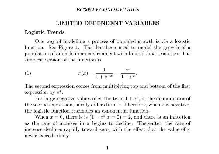
population of animals in an environment with limited food resources. The simplest version of the function is (1) π(x) = 1 1 + e−x = ex 1 + ex . The second expression comes from multiplying top and bottom of the first expression by ex. For large negative values of x, the term 1 + ex, in the denominator of the second expression, hardly differs from 1. Therefore, when x is negative, the logistic function resembles an exponential function. When x = 0, there is is (1 + ex|x = 0) = 2, and there is an inflection as the rate of increase in π begins to decline. Thereafter, the rate of increase declines rapidly toward zero, with the effect that the value of π never exceeds unity. 1
SLIDE 2 EC3062 ECONOMETRICS The inverse mapping x = x(π) is easily derived. Consider (2) 1 − π = 1 + ex 1 + ex − ex 1 + ex = 1 1 + ex = π ex . This is rearranged to give (3) ex = π 1 − π , whence the inverse function is found by taking natural logarithms: (4) x(π) = ln
1 − π
2
SLIDE 3
EC3062 ECONOMETRICS 0.25 0.5 1.0 −4 −2 2 4
Figure 1. The logistic function ex/(1 + ex) and its derivative. For large negative values of x, the function and its derivative are close. In the case of the exponential function ex, they coincide for all values of
x. 3
SLIDE 4 EC3062 ECONOMETRICS The logistic curve needs to be elaborated before it can be fitted flexi- bly to a set of observations y1, . . . , yn tending to an upper asymptote. The general from of the function is (5) y(t) = γ 1 + e−h(t) = γeh(t) 1 + eh(t) ; h(t) = α + βt. Here γ is the upper asymptote of the function, and β and α determine the rate of ascent of the function and the mid point of its ascent. It can be seen that (6) ln
γ − y(t)
With the inclusion of a residual term, the equation bcomes (7) ln
γ − yt
For a given value of γ, one may calculate the value of the dependent variable on the LHS. Then the values of α and β may be found by least- squares regression. 4
SLIDE 5 EC3062 ECONOMETRICS The value of γ may also be determined according to the criterion of minimising the sum of squares of the residuals. A crude procedure would entail running numerous regressions, each with a different value for γ. The definitive value would be the one from the regression with the least residual sum of squares. There are other procedures for finding the minimising value of γ
- f a more systematic and efficient nature which might be used instead.
Amongst these are the methods of Golden Section Search and Fibonnaci Search which are presented in many texts of numerical analysis. The objection may be raised that the domain of the logistic function is the entire real line—which spans all of time from creation to eternity— whereas the sales history of a consumer durable dates only from the time when it is introduced to the market. The problem might be overcome by replacing the time variable t in equation (15) by its logarithm and by allowing t to take only nonnegative values. See Figure 2. Then, whilst t ∈ [0, ∞), we still have ln(t) ∈ (−∞, ∞), which is the entire domain of the logistic function. 5
SLIDE 6
EC3062 ECONOMETRICS 1 2 3 4 0.2 0.4 0.6 0.8 1.0
Figure 2. The function y(t) = γ/(1 + exp{α − β ln(t)}) with
γ = 1, α = 4 and β = 7. The positive values of t are the domain of
the function.
6
SLIDE 7 EC3062 ECONOMETRICS 0.5 1.0 1.5 2.0 2.5 3.0 0.2 0.4 0.6 0.8 1.0
Figure 3. The cumulative log-normal distribution. The logarithm
- f the log-normal variate is a standard normal variate.
7
SLIDE 8 EC3062 ECONOMETRICS A Binary Dependent Variable: A Probit Model in Biology Consider the effects of a pesticide on a sample of insects. For the ith insect, the lethal dosage is the quantity δi, with log(δi) = λi ∼ N(λ, σ2). If an insect is selected at random and is subjected to the dosage di, then the probability that it will die is P(λi ≤ xi), where xi = log(di). The probability is (8) π(xi) = xi
−∞
N(ζ; λ, σ2)dζ. The function π(xi) with xi = log(di) also indicates the fraction of the insects expected to die when all the individuals were subjected to the same global dosage d = di. Let yi = 1 if the ith insect dies and yi = 0 if it survives. Then the situation of the ith insect is summarised by (9) yi = 0, if λi > xi
δi > di; 1, if λi ≤ xi
δi ≤ di. 8
SLIDE 9 EC3062 ECONOMETRICS The integral of (8) may be expressed in terms of a standard normal density function N(ε; 0, 1). Thus (10) P(λi < xi) with λi ∼ N(λ, σ2) is equal to P λi − λ σ = εi < hi = xi − λ σ
εi ∼ N(0, 1). Moreover, the standardised variable hi, which corresponds to the dose received by the ith insect, can be written as (11) hi = xi − λ σ = β0 + β1xi, where β0 = −λ σ and β1 = 1 σ . To fit the model to the data, it is necessary only to estimate the parameters λ and σ2 of the normal probability density function or, equivalently, to estimate the parameters β0 and β1. 9
SLIDE 10
EC3062 ECONOMETRICS ξi, λi ξi y, 1 − π y = 0 y = 1 λi
* λ
0.3
Figure 4. The probability of the threshold λi ∼ N(λ, σ2) falling short of the realised value λ∗
i is the area of the shaded region in the lower diagram.
10
SLIDE 11
EC3062 ECONOMETRICS The Probit Model in Econometrics If the stimulus ξi exceeds the realised threshold λ∗
i , then the step
function, indicated by the arrows in the upper diagram, delivers y = 1. The upper diagram also shows the cumulative probability distribution function, which indicates a probability value of P(λi < λ∗
i ) = 1 − πi = 0.3
In econometrics, the Probit model is commonly used in describing binary choices. The systematic influences affecting the outcome for the ith consumer may be represented by a function ξi = ξ(x1i, . . . , xni), which may be a linear combination of the variables. The idiosyncratic effects can be represented by a normal random variable of zero mean. The ith individual will have a positive response yi = 1 only if the stimulus ξi exceeds their own threshold value λi ∼ N(λ, σ2), which is assumed to deviate at random from the level of a global threshold λ. Otherwise, there will be no response, indicated by yi = 0. Thus (12) yi = 0, if λi > ξi; 1, if λi ≤ ξi. These circumstances are illustrated in Figure 4. 11
SLIDE 12 EC3062 ECONOMETRICS The accompanying probability statements, expressed in term of a standard normal variate, are that (13) P(yi = 0|ξi) = P λi − λ σ = −εi > ξi − λ σ
P(yi = 1|ξi) = P λi − λ σ = −εi ≤ ξi − λ σ
where εi ∼ N(0, 1). On the assumption that ξ = ξ(x1, . . . , xn) is a linear function, these can be written as (14) P(yi = 0) = P (0 > y∗
i = β0 + xi1β1 + · · · + xikβk + εi)
and P(yi = 1) = P (0 ≤ y∗
i = β0 + xi1β1 + · · · + xikβk + εi) ,
where β0 + xi1β1 + · · · + xikβk = ξ(x1i, . . . , xki) − λ σ . Thus, the original statements relating to the distribution N(λi; λ, σ2) can be converted to equivalent statements expressed in terms of the standard normal distribution N(εi; 0, 1). 12
SLIDE 13 EC3062 ECONOMETRICS The essential quantities that require to be computed in the process
- f fitting the model to the data of the individual respondents, who are
indexed by i = 1, . . . , N, are the probability values (15) P(yi = 0) = 1 − πi = Φ(β0 + xi1β1 + · · · + xikβk), where Φ denotes the cumulative standard normal distribution function. These probability values depend on the coefficients β0, β1, . . . , βk of the linear combination of the variables influencing the response. Estimation with Individual Data Imagine that we have a sample of observations (yi, xi.); i = 1, . . . , N, where yi ∈ {0, 1} for all i. Then, assuming that the events affecting the individuals are statistically independent and taking πi = π(xi., β) to represent the probability that the event will affect the ith individual, we can write represent the likelihood function for the sample as (16) L(β) =
N
πyi
i (1 − πi)1−yi = N
1 − πi yi (1 − πi). 13
SLIDE 14 EC3062 ECONOMETRICS This is the product of n point binomials. The log of the likelihood function is given by (17) log L =
N
yi log
1 − πi
N
log(1 − πi). Differentiating log L with respect to βj, which is the jth element of the parameter vector β, yields (18) ∂ log L ∂βj =
N
yi πi(1 − πi) ∂πi ∂βj −
N
1 1 − πi ∂πi ∂βj =
N
yi − πi πi(1 − πi) ∂πi ∂βj . To obtain the second-order derivatives which are also needed, it is helpful to write the final expression of (20) as (19) ∂ log L ∂βj =
yi πi − 1 − yi 1 − πi ∂πi ∂βj . 14
SLIDE 15 EC3062 ECONOMETRICS Then it can be seen more easily that (20) ∂2 log L ∂βjβk =
yi πi − 1 − yi 1 − πi ∂2πi ∂βjβk −
yi π2
i
+ 1 − yi (1 − πi)2 ∂πi ∂βj ∂πi ∂βk . The negative of the expected value of the matrix of second derivatives is the information matrix whose inverse provides the asymptotic dispersion matrix of the maximum-likelihood estimates. The expected value of the expression above is found by taking E(yi) = πi. On taking expectations, the first term of the RHS of (20) vanishes and the second term is simplified, with the result that (21) E ∂2 log L ∂βjβk
1 πi(1 − πi) ∂πi ∂βj ∂πi ∂βk . The maximum-likelihood estimates are the values which satisfy the conditions (22) ∂ log L(β) ∂β = 0. 15
SLIDE 16
EC3062 ECONOMETRICS To solve this equation requires an iterative procedure. The Newton– Raphson procedure serves the purpose. The Newton–Raphson Procedure A common procedure for finding the solution or root of a nonlinear equation α(x) = 0 is the Newton–Raphson procedure which depends upon approximating the curve y = α(x) by its tangent at a point near the root. Let this point be [x0, α(x0)]. Then the equation of the tangent is (23) y = α(x0) + ∂α(x0) ∂x (x − x0) and, on setting y = 0, we find that this line intersects the x-axis at (24) x1 = x0 − ∂α(x0) ∂x −1 α(x0). If x0 is close to the root λ of the equation α(x) = 0, then we can expect x1 to be closer still. To find an accurate approximation to λ, we generate 16
SLIDE 17
EC3062 ECONOMETRICS a sequence of approximations {x0, x1, . . . , xr, xr+1, . . .} according to the algorithm (25) xr+1 = xr − ∂α(xr) ∂x −1 α(xr). The Newton–Raphson procedure is readily adapted to the problem of finding the value of the vector β which satisfies the equation ∂ log L(β)/∂β = 0, which is the first-order condition for the maximisation of the log- likelihood function. Let β consist of two elements β0 and β1. Then the algorithm by which the (r+1)th approximation to the solution is obtained from the rth approximation is specified by (26) β0 β1
(r+1)
= β0 β1
(r)
− ∂2 log L ∂β2 ∂2 log L ∂β0β1 ∂2 log L ∂β1β0 ∂2 log L ∂β2
1
−1 (r)
∂ log L ∂β0 ∂ log L ∂β1 . It is common to replace the matrix of second-order partial derivatives in this algorithm by its expected value which is the negative of information 17
SLIDE 18 EC3062 ECONOMETRICS x y x0 x1 x2
Figure 5. If x0 is close to the root of the equation
α(x) = 0, then we can expect x1 to be closer still.
- matrix. The modified procedure is known as Fisher’s method of scoring.
18
SLIDE 19
EC3062 ECONOMETRICS The algebra is often simplified by replacing the derivatives by their expec- tations, whereas the properties of the algorithm are hardly affected. In the case of the simple probit model, where there is no closed-form expression for the likelihood function, the probability values, together with the various derivatives and expected derivatives to be found under (18) to (21), which are needed in order to implement one or other of these estimation procedures, may be evaluated with the help of tables which can be read into the computer. Recall that the probability values π are specified by the cumulative normal distribution (27) π(h) = h
−∞
1 √ 2π e−ζ2/2dζ. We may assume, for the sake of a simple illustration, that the function h(x) is linear: (28) h(x) = β0 + β1x. 19
SLIDE 20
EC3062 ECONOMETRICS Then the derivatives ∂πi/∂βj become (29) ∂πi ∂β0 = ∂πi ∂h . ∂h ∂β0 = N{h(xi)} and ∂πi ∂β1 = ∂πi ∂h . ∂h ∂β1 = N{h(xi)}xi, where N denotes the normal density function which is the derivative of π. Estimation with Grouped Data In the classical applications of probit analysis, the data was usually in the form of grouped observations. Thus, to assess the effectiveness of an insecticide, various levels of dosage dj; j = 1, . . . , J would be administered to batches of nj insects. The numbers mj =
i yij killed in each batch
would be recorded and their proportions pj = mj/nj would be calculated. If a sufficiently wide range of dosages are investigated, and if the numbers nj in the groups are large enough to allow the sample proportions pj accurately to reflect the underlying probabilities πj, then the plot of pj against xj = log dj should give a clear impression of the underlying distribution function π = π{h(x)}. In the case of a single experimental variable x, it would be a simple matter to infer the parameters of the function h = β0 +β1x from the plot. 20
SLIDE 21 EC3062 ECONOMETRICS According to the model, we have (30) π(h) = π(β0 + β1x). From the inverse h = π−1(π) of the function π = π(h), one may obtain the values hj = π−1(pj). In the case of the probit model, this is a matter of referring to the table of the standard normal distribution. The values of π
- r p are found in the body of the table whilst the corresponding values of
h are the entries in the margin. Given the points (hj, xj) for j = 1, . . . J, it is a simple matter to fit a regression equation in the form of (31) hj = b0 + b1xj + ej. In the early days of probit analysis, before the advent of the electronic computer, such fitting was often performed by eye with the help of a ruler. To derive a more sophisticated and efficient method of estimating the parameters of the model, we may pursue a method of maximum-likelihood. This method is a straightforward generalisation of the one which we have applied to individual data. 21
SLIDE 22 EC3062 ECONOMETRICS Consider a group of n individuals which are subject to the same prob- ability P(y = 1) = π for the event in question. The probability that the event will occur in m out of n cases is given by the binomial formula: (32) B(m, n, π) = n m
n! m!(n − m)!πm(1 − π)n−m. If there are J independent groups, then the joint probability of their out- comes m1, . . . , mj is the product (33) L =
J
nj mj
j
(1 − πj)nj−mj =
J
nj mj πj 1 − πj mj (1 − πj)nj. Therefore the log of the likelihood function is (34) log L =
J
1 − πj
nj mj
Given that πj = π(xj., β), the problem is to estimate β by finding the value which satisfies the first-order condition for maximising the likelihood 22
SLIDE 23 EC3062 ECONOMETRICS function which is (35) ∂ log L(β) ∂β = 0. To provide a simple example, let us take the linear logistic model (36) π = eβ0+β1x 1 + eβ0+β1x . The so-called log-odds ratio is (37) log
1 − π
Therefore the log-likelihood function of (34) becomes (38) log L =
J
- j=1
- mj(β0 + β1xj) − nj log(1 − eβ0+β1xj) + log
nj mj
23
SLIDE 24 EC3062 ECONOMETRICS and its derivatives in respect of β0 and β1 are (39) ∂ log L ∂β0 =
1 + eβ0+β1xj
(mj − njπj), ∂ log L ∂β1 =
1 + eβ0+β1xj
xj(mj − njπj). The information matrix, which, together with the above derivatives, is used in estimating the parameters by Fisher’s method of scoring, is pro- vided by (40)
j mjπj(1 − πj)
- j mjxjπj(1 − πj)
- j mjxjπj(1 − πj)
- j mjx2
jπj(1 − πj)
24