EC3062 ECONOMETRICS ELEMENTARY REGRESSION ANALYSIS We shall - PowerPoint PPT Presentation

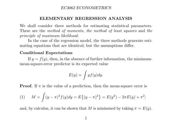
EC3062 ECONOMETRICS ELEMENTARY REGRESSION ANALYSIS We shall consider three methods for estimating statistical parameters. These are the method of moments, the method of least squares and the principle of maximum likelihood. In the case of the regression model, the three methods generate esti- mating equations that are identical; but the assumptions differ. Conditional Expectations If y ∼ f ( y ), then, in the absence of further information, the minimum- mean-square-error predictor is its expected value � E ( y ) = yf ( y ) dy. Proof. If π is the value of a prediction, then the mean-square error is � ( y − π ) 2 f ( y ) dy = E � ( y − π ) 2 � = E ( y 2 ) − 2 πE ( y ) + π 2 ; (1) M = and, by calculus, it can be shown that M is minimised by taking π = E ( y ). 1

EC3062 ECONOMETRICS If x is related to y , then the m.m.s.e prediction of y is the conditional expectation y f ( x, y ) � (2) E ( y | x ) = f ( x ) dy. Proof. Let ˆ y = E ( y | x ) and let π = π ( x ) be any other estimator. Then, �� � 2 � ( y − π ) 2 � � E = E ( y − ˆ y ) + (ˆ y − π ) (5) � y ) 2 � � � � y − π ) 2 � = E ( y − ˆ + 2 E ( y − ˆ y )(ˆ y − π ) + E (ˆ . In the second term, there is � � � � E ( y − ˆ y )(ˆ y − π ) = ( y − ˆ y )(ˆ y − π ) f ( x, y ) ∂y∂x x y (6) � � � � = ( y − ˆ y ) f ( y | x ) ∂y (ˆ y − π ) f ( x ) ∂x = 0 . x y Therefore, E { ( y − π ) 2 } = E { ( y − ˆ y ) 2 } + E { (ˆ y − π ) 2 } ≥ E { ( y − ˆ y ) 2 } , and the assertion is proved. 2

EC3062 ECONOMETRICS The definition of the conditional expectation implies that � � � � � � E ( xy ) = xyf ( x, y ) ∂y∂x = x yf ( y | x ) ∂y f ( x ) ∂x = E ( x ˆ y ) . x y x y � � When E ( xy ) = E ( x ˆ y ) is rewritten as E x ( y − ˆ y ) = 0 , it may be described as an orthogonality condition. This indicates that the prediction error y − ˆ y is uncorrelated with x . If it were correlated with x , then we should not be using the information of x efficiently in forming ˆ y . Linear Regression Assume that x and y have a joint normal distribution, which implies that there is a linear regression relationship: (9) E ( y | x ) = α + βx, The object is to express α and β in terms of the expectations E ( x ), E ( y ), the variances V ( x ), V ( y ) and the covariance C ( x, y ). 3

EC3062 ECONOMETRICS First, multiply (9) by f ( x ), and integrate with respect to x to give (10) E ( y ) = α + βE ( x ) , whence the equation for the intercept is (11) α = E ( y ) − βE ( x ) . Equation (10) shows that the regression line passes through the expected value of the joint distribution E ( x, y ) = { E ( x ) , E ( y ) } . By putting (11) into E ( y | x ) = α + βx from (9), we find that � � (12) E ( y | x ) = E ( y ) + β x − E ( x ) . Now multiply (9) by x and f ( x ) and integrate with respect to x to give E ( xy ) = αE ( x ) + βE ( x 2 ) . (13) Multiplying (10) by E ( x ) gives � 2 , � (14) E ( x ) E ( y ) = αE ( x ) + β E ( x ) 4

EC3062 ECONOMETRICS E ( xy ) = αE ( x ) + βE ( x 2 ) . (13) Multiplying (10) by E ( x ) gives � 2 , � (14) E ( x ) E ( y ) = αE ( x ) + β E ( x ) whence, on taking (14) from (13), we get � � 2 � E ( x 2 ) − � (15) E ( xy ) − E ( x ) E ( y ) = β E ( x ) , which implies that �� �� �� E x − E ( x ) y − E ( y ) (16) β = E ( xy ) − E ( x ) E ( y ) = C ( x, y ) � 2 = V ( x ) . �� � 2 � � E ( x 2 ) − E ( x ) E x − E ( x ) Thus, we have expressed α and β in terms of the moments E ( x ), E ( y ), V ( x ) and C ( x, y ) of the joint distribution of x and y . 5

EC3062 ECONOMETRICS Estimation by the Method of Moments Let ( x 1 , y 1 ) , ( x 2 , y 2 ) , . . . , ( x T , y T ) be a sample of T observations. Then, we can calculate the following empirical or sample moments: T T x = 1 y = 1 � � ¯ x t , ¯ y t , T T t =1 t =1 T T x = 1 x ) 2 = 1 � � s 2 x 2 x 2 , (21) ( x t − ¯ t − ¯ T T t =1 t =1 T T s xy = 1 y ) = 1 � � ( x t − ¯ x )( y t − ¯ x t y t − ¯ x ¯ y. T T t =1 t =1 To estimate α and β , we replace the population moments in the formulae of (11) and (16) by the sample moments. Then, the estimates are � ( x t − ¯ x )( y t − ¯ y ) y − ˆ ˆ (22) α = ¯ ˆ β ¯ x, β = . � ( x t − ¯ x ) 2 6

EC3062 ECONOMETRICS Convergence We can expect the sample moments to converge to the true moments of the bivariate distribution, thereby causing the estimates of the param- eters to converge likewise to the true values. (23) A sequence of numbers { a n } is said to converge to a limit a if, for any arbitrarily small real number ǫ , there exists a corresponding integer N such that | a n − a | < ǫ for all n ≥ N . This is not appropriate to a stochastic sequence, such as a sequence of estimates. For, it is always possible for a n to break the bounds of a ± ǫ when n > N . The following is a more appropriate definition: (24) A sequence of random variables { a n } is said to converge weakly in probability to a limit a if, for any ǫ , there is lim P ( | a n − a | > ǫ ) = 0 as n → ∞ or, equivalently, lim P ( | a n − a | ≤ ǫ ) = 1. With the increasing size of the sample, it becomes virtually certain that a n will ‘fall within an epsilon of a .’ We describe a as the probability limit of a n and we write plim( a n ) = a . 7

EC3062 ECONOMETRICS This definition does not presuppose that a n has a finite variance or even a finite mean. However, if a n does have finite moments, then we may talk of mean-square convergence: (25) A sequence of random variables { a n } is said to converge in mean square to a limit a if lim( n → ∞ ) E { ( a n − a ) 2 } = 0. We should note that ��� �� 2 � �� � 2 � � � E a n − a = E a n − E ( a n ) − a − E ( a n ) (26) �� � 2 � = V ( a n ) + E a − E ( a n ) . Thus, the mean-square error of an estimator a n is the sum of its variance and the square of its bias. If a n is to converge in mean square to a , then both of these quantities must vanish. Convergence in mean square implies convergence in probability. When an estimator converges in probability to the parameter which it purports to represent, then we say that it is a consistent estimator. 8

EC3062 ECONOMETRICS 80 75 70 65 60 55 55 60 65 70 75 80 Figure 1. Pearson’s data comprising 1078 measurements of the heights of fathers (the abscissae) and of their sons (the ordinates), together with the two regression lines. The correlation coefficient is 0.5013. 9

EC3062 ECONOMETRICS The Bivariate Normal Distribution Most of the results in the theory of regression can be obtained by examining the functional form of the bivariate normal distribution. Let x and y be the two variables. Let us denote their means by E ( x ) = µ x , E ( y ) = µ y , their variances by V ( x ) = σ 2 x , V ( y ) = σ 2 y and their covariance by C ( x, y ) = ρσ x σ y . Here, the correlation coefficient C ( x, y ) (30) ρ = � V ( x ) V ( y ) provides a measure of the relatedness of these variables. The bivariate distribution is specified by 1 (31) f ( x, y ) = 1 − ρ 2 exp Q ( x, y ) , � 2 πσ x σ y where (32) �� x − µ x � 2 � � 2 − 1 � x − µ x � � y − µ y � � y − µ y Q = − 2 ρ + . 2(1 − ρ 2 ) σ x σ x σ y σ y 10

EC3062 ECONOMETRICS The quadratic function can also be written as �� y − µ y � 2 � � 2 � x − µ x − 1 − ρx − µ x − (1 − ρ 2 ) (33) Q = . 2(1 − ρ 2 ) σ y σ x σ x Thus, we have (34) f ( x, y ) = f ( y | x ) f ( x ) , where − ( x − µ x ) 2 1 � � √ (35) f ( x ) = 2 π exp , 2 σ 2 σ x x and − ( y − µ y | x ) 2 1 � � (36) f ( y | x ) = exp , � 2 σ 2 y (1 − ρ ) 2 σ y 2 π (1 − ρ 2 ) with µ y | x = µ y + ρσ y (37) ( x − µ x ) . σ x 11

EC3062 ECONOMETRICS Least-Squares Regression Analysis The regression equation, E ( y | x ) = α + βx can be written as (39) y = α + xβ + ε, where ε = y − E ( y | x ) is a random variable, with E ( ε ) = 0 and V ( ε ) = σ 2 , that is independent of x . Given observations ( x 1 , y 1 ) , . . . , ( x T , y T ), the estimates are the values that minimise the sum of squares of the distances—measured parallel to the y -axis—of the data points from an interpolated regression line: T T � � ε 2 ( y t − α − x t β ) 2 . (40) S = t = t =1 t =1 Differentiating S with respect to α and setting to zero gives � (41) − 2 ( y t − α − βx t ) = 0 , or y − α − β ¯ ¯ x = 0 . This generates the following estimating equation for α : (42) α ( β ) = ¯ y − β ¯ x. 12

EC3062 ECONOMETRICS By differentiating with respect to β and setting the result to zero, we get � (43) − 2 x t ( y t − α − βx t ) = 0 . On substituting for α from (42) and eliminating the factor − 2, this be- comes � � � x 2 (44) x t y t − x t (¯ y − β ¯ x ) − β t = 0 , whence we get � x t y t − T ¯ � ( x t − ¯ x ¯ y x )( y t − ¯ y ) ˆ � x 2 (45) β = = . t − T ¯ x 2 � ( x t − ¯ x ) 2 This is identical to the estimate under (22) derived via the method of moments. Putting ˆ β into the equation α ( β ) = ¯ y − β ¯ x of (42), gives the estimate of ˆ α found under (22). 13