EC3062 ECONOMETRICS MATRIX KRONECKER PRODUCTS Consider the matrix - PowerPoint PPT Presentation

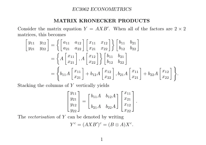
EC3062 ECONOMETRICS MATRIX KRONECKER PRODUCTS Consider the matrix equation Y = AXB ′ . When all of the factors are 2 × 2 matrices, this becomes � � �� � � �� � � y 11 y 12 a 11 a 12 x 11 x 12 b 11 b 21 = y 21 y 22 a 21 a 22 x 21 x 22 b 12 b 22 � � � � �� � � x 11 x 12 b 11 b 21 = A , A x 21 x 22 b 12 b 22 � � � � � � � � � � x 11 x 12 x 11 x 12 = b 11 A + b 12 A , b 21 A + b 22 A . x 21 x 22 x 21 x 22 Stacking the columns of Y vertically yields y 11 x 11 � b 11 A   �   b 12 A y 21 x 21  =  .     y 12 x 12   b 21 A b 22 A y 22 x 22 The vectorisation of Y can be denoted by writing Y c = ( AXB ′ ) c = ( B ⊗ A ) X c . 1

EC3062 ECONOMETRICS The Kronecker product of the matrices A and B is defined by a 11 B a 11 B . . . a 1 n B   a 21 B a 21 B . . . a 2 m B   A ⊗ B =  . . . .  . . .  . . .  a m 1 B a m 2 B . . . a mn B The following rules govern Kronecker products: (i) ( A ⊗ B )( C ⊗ D ) = AC ⊗ BD, ( A ⊗ B ) ′ = A ′ ⊗ B ′ , (ii) (iii) A ⊗ ( B + C ) = ( A ⊗ B ) + ( A ⊗ C ) , (iv) λ ( A ⊗ B ) = λA ⊗ B = A ⊗ λB, ( A ⊗ B ) − 1 = ( A − 1 ⊗ B − 1 ) . (v) The product is non-commutative, which is to say that A ⊗ B � = B ⊗ A . However, observe that A ⊗ B = ( A ⊗ I )( I ⊗ B ) = ( I ⊗ B )( A ⊗ I ) . 2

EC3062 ECONOMETRICS ECONOMETRIC PANEL DATA The Unrestricted Model with Common Regressors Consider M firms or individuals indexed by j = 1 , . . . , M . These react differ- ently to the same measured influences, as indicated by the parameters α j and β .j . The set of T realisations of the j th equation can be written as (8) y .j = α j ι T + Xβ .j + ε .j . This is a classical regression equation that can be estimated by OLS. The full set of M such equations can be compiled as the system: y . 1 β . 1 ι T 0 . . . 0 α 1 ε . 1 X 0 . . . 0             y . 2 0 ι T . . . 0 α 2 β . 2 ε . 2 0 X . . . 0              =  + . . .  +  . . . . . . ... . . ... . . .    . . .   .       .  . . . . . . . . . . . .         0 0 . . . X 0 0 . . . ι T α M ε .M y .M β .M Using the Kronecker product, this can be rendered as Y c = ( I M ⊗ ι T ) α + ( I M ⊗ X ) B c + E c . (10) 3

EC3062 ECONOMETRICS The General Model A useful elaboration is to allow the matrix X to vary between the M equations. Then, in place of the variables x tk , there are elements x tkj bearing the individual-specific subscript j . Then, equation (9) is replaced by y . 1 ι T 0 . . . 0 α 1       y . 2 0 ι T . . . 0 α 2        = . . . . . ...    . . .   .  . . . . . .      0 0 . . . ι T α M y .M (11) β . 1 X 1 0 . . . 0 ε . 1       β . 2 0 X 2 . . . 0 ε . 2       +  +  . . . . . . ...       . . . . . . . . . .     0 0 . . . X M β .M ε .M For example, the equations, explaining farm production in M regions, may com- prise explanatory variables whose measured values vary from region to region. The j th equation of the general model can be written as (12) y .j = ι T α j + X j β.j + ε .j . 4

EC3062 ECONOMETRICS The Model with Individual Fixed Effects Within this model, some restrictions can be imposed. Thus (13) H β : β . 1 = β . 2 = · · · = β .M , asserts that the slope parameters of all M of the regression equations are equal. This condition gives rise to the following model: y . 1 ι T 0 . . . 0 α 1 X 1 ε . 1           y . 2 0 ι T . . . 0 α 2 X 2 ε . 2           (14)  =  +  β +  , . . . . . . . ...    . . .   .   .   .  . . . . . . . .       y .M 0 0 . . . ι T α M X M ε .M Here, each of the M equations has a particular value for the intercept. This system of equations can be rendered as Y c = ( I M ⊗ ι T ) α + Xβ + E c , (15) where X ′ = [ X ′ 1 , X ′ 2 , . . . , X ′ M ]. It is common, in many many textbooks, to write ( I M ⊗ ι T ) = D for the so-called matrix of dummy variables associated with the intercept terms. 5

EC3062 ECONOMETRICS The Pooled Model A further hypothesis is that all of the intercepts have the same value: (16) H α : α 1 = α 2 = · · · = α M . It is unlikely that one would maintain this hypothesis without asserting H β at the same time. The combined hypothesis H γ = H α ∩ H β gives rise to y . 1 ι T X 1 ε . 1         y . 2 ι T X 2 ε . 2         (17)  =  α +  β +  . . . . .    .   .   .  . . . . .     ι T X M ε .M y .M This system of equations can be rendered as Y c = ι MT α + Xβ + E c , (18) where, as before, X ′ = [ X ′ 1 , X ′ 2 , . . . , X ′ M ] and where ι MT is a long vector consist- ing of MT units. This has the structure of the equation of a classical regression model, for which OLS is efficient. 6

EC3062 ECONOMETRICS The Least-Squares Estimation: the General Unrestricted Model We assume that the disturbances ε tj are distributed independently and identically, with E ( ε tj ) = 0 and V ( ε tj ) = σ 2 for all t, j . Then, the equations of the general model of (11) are separable, and the j th equation may be estimated efficiently by OLS. The regression can be applied directly to the individual equations of (11). Alternatively, the intercept terms can be eliminated by taking the deviations of the data about their respective sample means. Then, the estimates for the j th equation are � − 1 X ′ ˆ � X ′ β .j = j ( I − P T ) X j j ( I − P T ) y .j and (19) x j. ˆ α j = ¯ ˆ y j − ¯ β .j , where T ι T ) − 1 ι ′ I − P T = I − ι T ( ι ′ (20) T is the operator that transforms a vector of T observations into the vector of their deviations about the mean. 7

EC3062 ECONOMETRICS The intercept terms would be eliminated by premultiplying the full system of equations by W = I M ⊗ ( I T − P T ) = I MT − ( I M ⊗ P T ) (24) = I MT − D ( D ′ D ) − 1 D ′ . The residual sum of squares from the j th regression is given by j ( I − P T ) X j } − 1 X ′ S j = y ′ .j ( I − P T ) y .j − y ′ .j ( I − P T ) X j { X ′ (21) j ( I − P T ) y .j . From the separability of the M regressions, it follows that the residual sum of squares, obtained from fitting the multi-equation model of (11) to the data, is � (22) S = S j . j 8

EC3062 ECONOMETRICS Estimation of the Model with Individual Fixed Effects Now, consider fitting the model under (14), which arises from the general model (11) when the slope parameters of the regressions are the same in every region. Then, the efficient estimates are obtained by treating the system of equations as a whole. To eliminate the intercept terms, the individual equations y .j = α j ι T + X j β + ε j are multiplied by the operator I − P T , to create deviations of the data about sample means: (25) ( I − P T ) y .j = ( I − P T ) X j β + ( I − P T ) ε j , The equation at time t is (26) y tj − ¯ y j = ( x .tj − ¯ x .j ) β + ( ε tj − ¯ ε j ) . To obtain an efficient estimate of β , the full set of TM mean-adjusted equa- tions must be taken together. Once the estimate of β available, the individual intercept terms can be obtained. 9

EC3062 ECONOMETRICS The efficient system-wide estimates for the slope parameters and the intercepts are � − 1 � � � � � ˆ X ′ X ′ β W = j ( I − P T ) X j j ( I − P T ) y j j j (27) � − 1 � X ′ � � X ′ � � = I M ⊗ ( I T − P T ) X I M ⊗ ( I T − P T ) y and x j ˆ α j = ¯ ˆ y j. − ¯ β W , j = 1 , . . . , M, where X ′ = [ X ′ M ] and y ′ = [ y ′ .M ]. Here, ˆ 1 , X ′ 2 , . . . , X ′ . 1 y ′ . 2 , . . . , y ′ β W is the result of applying OLS to an equation derived by premultiplying (14) by the matrix W of (24), to annihilate the intercept terms. The residual sum of squares from fitting the model of (14) is given by S β = y ′ Wy − y ′ WX ( X ′ WX ) − 1 X ′ Wy, where (28) W = I M ⊗ ( I T − P T ) . The estimator ˆ β W of (27) makes use only of the information conveyed by the deviations of the data points from their means within the M groups. For this reason, it is often called the within-groups estimator. 10