SLIDE 1 EC3062 ECONOMETRICS DYNAMIC REGRESSIONS MODELS Autoregressive Disturbance Processes Economic variables often follow slowly-evolving trends and they tend to be strongly correlated with each other. If the disturbance term is compounded from such variables, then it should have similar characteristics. In the classical model, the disturbances ε(t) = {εt; t = 0, ±1, ±2, . . .} are independently and identically distributed such that (2) E(εt) = 0, for all t and C(εt, εs) =
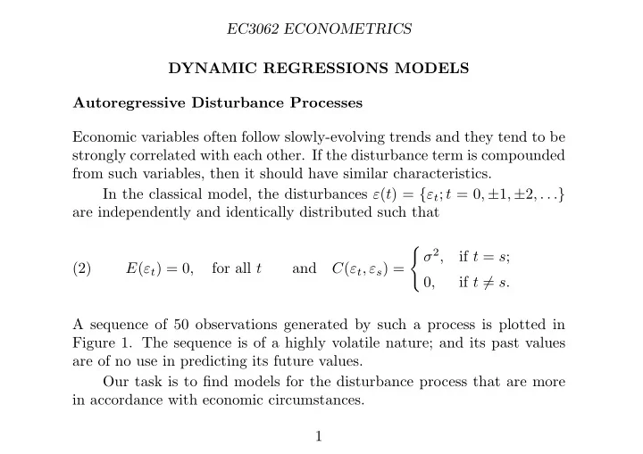
if t = s; 0, if t = s. A sequence of 50 observations generated by such a process is plotted in Figure 1. The sequence is of a highly volatile nature; and its past values are of no use in predicting its future values. Our task is to find models for the disturbance process that are more in accordance with economic circumstances. 1
SLIDE 2
EC3062 ECONOMETRICS 0.0 0.5 1.0 1.5 2.0 2.5 0.0 −0.5 −1.0 −1.5 −2.0 10 20 30 40 50 Figure 1. 50 observations on a white-noise process ε(t) of unit variance. 2
SLIDE 3 EC3062 ECONOMETRICS The traditional means of representing the inertial properties of the distur- bance process has been to adopt a simple first-order autoregressive model,
- r AR(1) model, whose equation takes the form of
(3) ηt = φηt−1 + εt, where φ ∈ (−1, 1). In many econometric applications, the value of φ falls in the more restricted interval [0, 1). The conditional expectation of ηt given ηt−1 is E(ηt|ηt−1) = φηt−1. If φ is close to unity, there will be a high degree of correlation amongst successive elements of η(t) = {ηt; t = 0, ±1, ±2, . . .}. Figure 2 shows 50
- bservations on an AR(1) process with φ = 0.9
The covariance of two elements of the sequence η(t) that are separated by τ time periods is given by (4) C(ηt−τ, ηt) = γτ = σ2 φτ 1 − φ2 . Their correlation declines as their temporal separation increases. 3
SLIDE 4
EC3062 ECONOMETRICS 2 4 6 −2 10 20 30 40 50 Figure 2. 50 observations on an AR(1) process η(t) = 0.9η(t − 1) + ε(t). 4
SLIDE 5 EC3062 ECONOMETRICS Detecting Serial Correlation in the Regression Disturbances Imagine that the sequence η(t) = {ηt; t = 0, ±1, ±2, . . .} of the regression disturbances follows an AR(1) process such that (12) η(t) = ρη(t − 1) + ε(t), with ρ ∈ [0, 1). If this could be observed directly, then the serial correlation could be de- tected by testing the significance of the estimate of ρ, which is (13) h = T
t=2 ηt−1ηt
T
t=1 η2 t
. When residuals are used in the place of disturbances, this will be affected, in finite samples, by the values of the explanatory variables. The traditional approach to testing for serial correlation is due to Durbin and Watson. They have attempted to make an explicit allowance for the uncertainties that arise from not knowing the precise distribution
- f the test statistic in any particular instance.
5
SLIDE 6 EC3062 ECONOMETRICS The test statistic of Durbin and Watson, which is based upon the sequence {et; t = 1, 2, . . . , T} of ordinary least-square residuals, is defined by (14) d = T
t=2(et − et−1)2
T
t=1 e2 t
. This statistic may be used for detecting any problem of misspecification indicated by seeming violations of the assumption of i.i.d disturbances. Expanding the numerator of the D–W statistic, we find that (15) d = 1 T
t=1 e2 t
T
e2
t − 2 T
etet−1 +
T
e2
t−1
where (16) r = T
t=2 etet−1
T
t=1 e2 t
is an estimate of the coefficient ρ of serial correlation based on the ordinary least-squares residuals. 6
SLIDE 7 EC3062 ECONOMETRICS If ρ and likewise r are close to 1, then d will be close to zero; and there is a strong indication of serial correlation. If ρ is close to zero, so that the i.i.d assumption is more or less valid, then d will be close to 2. Given that their statistic is based on residuals rather than on distur- bances, Durbin and Watson provided a table of critical values that included a region of indecision. Their decision rules are as follows: if d < dL, then acknowledge the presence of serial correlation, if dL ≤ d ≤ dU, then remain undecided, if dU < d, then deny the presence of serial correlation. The values of dL and dU in the table depend on sample size and the number
- f variables included in the regression, not counting the intercept term.
As the number of degrees of freedom increases, the region of indecision lying between dL and dU becomes smaller, until a point is reached were it is no longer necessary to make any allowance for it. 7
SLIDE 8
EC3062 ECONOMETRICS Estimating a Regression Model with AR(1) Disturbances Assume that the regression equation takes the form of (18) y(t) = α + βx(t) + η(t), with η(t) = ρη(t − 1) + ε(t). Subtracting ρy(t−1) = ρα+ρβx(t−1)+ρε(t−1), and using Lx(t) = x(t−1), Ly(t) = y(t − 1) and Lε(t) = ε(t − 1), gives (21) (1 − ρL)y(t) = (1 − ρL)α + (1 − ρL)βx(t) + ε(t) = µ + (1 − ρL)βx(t) + ε(t), where µ = (1 − ρ)α. On defining the transformed variables, (23) q(t) = (1 − ρL)y(t) and w(t) = (1 − ρL)x(t). this can be written as (22) q(t) = µ + βw(t) + ε(t), 8
SLIDE 9 EC3062 ECONOMETRICS If a value is given to ρ, then we can form (25) q2 = y2 − ρy1, q3 = y3 − ρy2, . . . qT = yT − ρyT −1, w2 = x2 − ρx1, w3 = x3 − ρx2, . . . wT = xT − ρxT −1, and the equations (26) qt = µ + βwt + ut; t = 2, . . . , T can be subjected to an ordinary least-squares regression. The regression can be repeated for various values of ρ; and the definitive estimates of ρ, α = µ/(1 − α) and β are those corresponding to the minimum of the residual sum of squares. The procedure of searching for the optimal value of ρ may be conducted in a systematic manner using a line-search algorithm such as the method
- f Fibonacci Search or the method of Golden-Section Search, which are
described in textbooks of numerical optimisation. 9
SLIDE 10 EC3062 ECONOMETRICS In the Cochrane–Orcutt method, ρ is estimated via a subsidiary regression. The method is an iterative one in which each stage comprises two ordinary least-squares regressions. Given an initial value for ρ, the parameters µ and β are determined from (27) yt − ρyt−1 = µ + β(xt − ρxt−1) + εt
qt = µ + βwt + εt. Given values for β and α = µ/(1−ρ), a revised value for ρ can be determined via a second regression applied to (28) (yt − α − βxt) = ρ(yt−1 − α − βxt−1) + εt
ηt = ρηt−1 + εt. The revised value of ρ can fed back into equation (27), from which revised values of α and β can be obtained. The procedure can be pursued through successive iterations, until it converges. 10
SLIDE 11
EC3062 ECONOMETRICS The Feasible Generalised Least-Squares Estimator The search procedure and the Cochrane–Orcutt procedure can be viewed within the context of the generalised least-squares (GLS) estimator that takes account of the dispersion matrix of the vector of disturbances. The efficient GLS estimator of β in the model (y; Xβ, σ2Q) is (31) β∗ = (X′Q−1X)−1X′Q−1y. The dispersion matrix of the vector η = [η1, η2, η3, . . . ηT ]′, generated by an AR(1) process is [γ|i−j|] = σ2
εQ, where
(29) Q = 1 1 − φ2 ⎡ ⎢ ⎢ ⎢ ⎢ ⎣ 1 φ φ2 . . . φT −1 φ 1 φ . . . φT −2 φ2 φ 1 . . . φT −3 . . . . . . . . . ... . . . φT −1 φT −2 φT −3 . . . 1 ⎤ ⎥ ⎥ ⎥ ⎥ ⎦ . 11
SLIDE 12
EC3062 ECONOMETRICS It can be confirmed directly that (30) Q−1 = ⎡ ⎢ ⎢ ⎢ ⎢ ⎢ ⎢ ⎣ 1 −φ . . . −φ 1 + φ2 −φ . . . −φ 1 + φ2 . . . . . . . . . . . . ... . . . . . . . . . 1 + φ2 −φ . . . −φ 1 ⎤ ⎥ ⎥ ⎥ ⎥ ⎥ ⎥ ⎦ . Given its sparsity, the matrix Q−1 could be used directly in implementing the GLS estimator for which the formula is (31) β∗ = (X′Q−1X)−1X′Q−1y. By exploiting the factorisation Q−1 = T ′T, the estimates can be ob- tained by applying OLS to the transformed data W = TX and g = Ty. Thus, it can be seen that (32) β∗ = (W ′W)−1W ′g = (X′T ′TX)−1X′T ′Ty = (X′Q−1X)−1X′Q−1y. 12
SLIDE 13 EC3062 ECONOMETRICS The factor T of the matrix Q−1 = T ′T takes the form of (33) T = ⎡ ⎢ ⎢ ⎢ ⎢ ⎢ ⎣
. . . −φ 1 . . . −φ 1 . . . . . . . . . . . . ... . . . . . . 1 ⎤ ⎥ ⎥ ⎥ ⎥ ⎥ ⎦ . This effects a simple transformation of the data. The element y1 within y = [y1, y2, y3, . . . , yT ]′ is replaced y1
- 1 − φ2, whereas yt is replaced by
yt − φyt−1, for all t > 1. Since ρ must be estimated by one or other of the methods that we have outlined above, the resulting estimator of β is apt to be described as a feasible GLS estimator. The true GLS estimator, which would require a precise knowledge of ρ, is an infeasible estimator. 13
SLIDE 14 EC3062 ECONOMETRICS Distributed Lags In the early days of econometrics, attempts were made to model the dy- namic responses primarily by including lagged values of x on the RHS of the regression equation; and the so-called distributed-lag model was commonly adopted, which takes the form of (34) y(t) = β0x(t) + β1x(t − 1) + · · · + βkx(t − k) + ε(t). Here, the sequence of coefficients {β0, β1, . . . , βk} constitutes the impulse- response function of the mapping from x(t) to y(t). That is to say, if we imagine that, on the input side, the signal x(t) is a unit impulse of the form (35) x(t) =
- . . . , 0, 1, 0, . . . , 0, 0 . . .}
which has zero values at all but one instant, then the output of the transfer function would be (36) r(t) =
- . . . , 0, β0, β1, . . . , βk, 0, . . .
- .
14
SLIDE 15 EC3062 ECONOMETRICS Another concept that helps in understanding the dynamic response is the step-response of the transfer function. Imagine that the input sequence is zero-valued up to a point in time when it assumes a constant unit value: (37) x(t) =
- . . . , 0, 1, 1, . . . , 1, 1 . . .}.
The output of the transfer function would be the sequence (38) s(t) =
- . . . , 0, s0, s1, . . . , sk, sk, . . .
- ,
where (39) s0 = β0, s1 = β0 + β1, . . . sk = β0 + β1 + · · · + βk. Here, the value sk, which is attained by the sequence when the full adjust- ment has been accomplished after k periods, is called the (steady-state) gain of the transfer function; and it is denoted by γ = sk. 15
SLIDE 16 EC3062 ECONOMETRICS The distributed-lag formulation of equation (34) is profligate in its use of parameters; and, given that the sequence x(t) is likely to show strong serial correlation, we may expect to encounter problems of multicollinearity. The Geometric Lag Structure Another early approach to the problem of defining a lag structure, which depends on two parameters β and φ, is the geometric lag scheme of Koyk: (40) y(t) = β
- x(t) + φx(t − 1) + φ2x(t − 2) + · · ·
- + ε(t).
The impulse-response function of the Koyk model is a geometrically de- clining sequence {β, φβ, φ2β, . . .} The gain of the transfer function, which is obtained by summing the geometric series, has the value of (41) γ = β 1 − φ. 16
SLIDE 17 EC3062 ECONOMETRICS By lagging the equation by one period and multiplying by φ, we get (42) φy(t − 1) = β
- φx(t − 1) + φ2x(t − 2) + φ3x(t − 3) + · · ·
- + φε(t − 1).
Taking the latter from (40) gives y(t) − φy(t − 1) = βx(t) +
(1 − φL)y(t) = βx(t) + (1 − φL)ε(t)
- f which the rational form is
(45) y(t) = β 1 − φLx(t) + ε(t). The following expansion can be used to recover equation (40): (46) β 1 − φLx(t) = β
- 1 + φL + φ2L2 + · · ·
- x(t)
= β
- x(t) + φx(t − 1) + φ2x(t − 2) + · · ·
- 17
SLIDE 18 EC3062 ECONOMETRICS Equation (43) cannot be estimated consistently by OLS regression because the composite disturbance term {ε(t) − φε(t − 1)} is correlated with the lagged dependent variable y(t − 1). A simple consistent estimation procedure is based on the equation under (40). The elements of y(t) within the sample may be expressed as (47) yt = β
∞
φixt−i + εt = θφt + β
t−1
φixt−i + εt = θφt + βzt + εt. Here (48) θ = β
- x0 + φx−1 + φ2x−2 + · · ·
- is a nuisance parameter, which embodies the presample elements of the
sequence x(t), whereas (49) zt = xt + φxt−1 + · · · + φt−1x1 is a synthetic variable based on the observations xt, xt−1, . . . , x1 and on the value attributed to φ. 18
SLIDE 19 EC3062 ECONOMETRICS The procedure for estimating φ and β that is based on equation (47) in- volves running a number of trial regressions with differing values of φ and, therefore, of the regressors φt and zt; t = 1, . . . , T. The definitive estimates are those that minimise the residual sum of squares. It is possible to elaborate this procedure so as to obtain the estimates
- f the parameters of the equation
(50) y(t) = β 1 − φLx(t) + 1 1 − ρLε(t), which has a first-order autoregressive disturbance scheme in place of the white-noise disturbance to be found in equation (45). The parameters φ and ρ may be estimated by searching within the square defined by −1 < ρ, φ < 1. The search might be confined to the quadrant defined by 0 ≤ ρ, φ < 1. One can afford, to ignore autoregressive nature of the disturbance pro- cess while searching for an optimum value for φ. When this has been found, the residuals will constitute estimates of the autoregressive disturbances, to which an AR(1) model can be fitted by OLS regression. 19
SLIDE 20 EC3062 ECONOMETRICS Lagged Dependent Variables A regression equation can also be set in motion by including lagged values
- f the dependent variable on the RHS. With one lagged value, we get
(51) y(t) = φy(t − 1) + βx(t) + ε(t). In terms of the lag operator, this is (52) (1 − φL)y(t) = βx(t) + ε(t),
- f which the rational form is
(53) y(t) = β 1 − φLx(t) + 1 1 − φLε(t). The advantage of equation (51) is that it is amenable to estimation by
- rdinary least-squares regression. Although the estimates will be biased in
finite samples, they will be consistent, if the model is correctly specified. The disadvantage is the restrictive assumption that the systematic and disturbance parts have the same dynamics. 20
SLIDE 21 EC3062 ECONOMETRICS Partial Adjustment and Adaptive Expectations A simple partial-adjustment model has the form (55) y(t) = λ
- γx(t)
- + (1 − λ)y(t − 1) + ε(t),
If y(t) is current consumption, x(t) is disposable income, then γx(t) = y∗(t) is “desired”consumption. If habits of consumption persist, then current consumption will be a weighted combination of the previous consumption and present desired consumption. The weights of the combination depend on the partial-adjustment pa- rameter λ ∈ (0, 1]. If λ = 1, then the consumers adjust their consumption instantaneously to the desired value. As λ → 0, their consumption habits become increasingly persistent. When the notation λγ = (1 − φ)γ = β and (1 − λ) = φ is adopted, equation (55) becomes identical to equation (51), which is the regression model with a lagged dependent variable. 21
SLIDE 22 EC3062 ECONOMETRICS According to Friedman’s Permanent Income Hypothesis, the consumption function is specified as y(t) = γx∗(t) + ε(t), where x∗(t) = (1 − φ)
- x(t) + φx(t − 1) + φ2x(t − 2) + · · ·
- = 1 − φ
1 − φLx(t) is the value of permanent or expected income, which is formed as a geo- metrically weighted sum of all past values of income. Observe that this is a case of adaptive expectations: x∗(t) = φx∗(t − 1) + (1 − φ)x(t). On substituting the expression for permanent income into the equation
- f the consumption function, we get
(59) y(t) = γ (1 − φ) 1 − φL x(t) + ε(t). When the notation γ(1−φ) = β is adopted, equation (59) becomes identical to the equation (45) of the Koyk model. 22
SLIDE 23 EC3062 ECONOMETRICS Error-Correction Forms, and Nonstationary Signals The usual linear regression procedures presuppose that the relevant moment matrices will converge asymptotically to fixed limits as the sample size increases. This cannot happen if the data are trended, in which case, the standard techniques of statistical inference will not be applicable. A common approach is to subject the data to as many differencing
- perations as may be required to achieve stationarity. However, differencing
tends to remove some of the essential information regarding the behaviour
- f economic agents. Moreover, it is often discovered that the regression
model looses much of its explanatory power when the differences of the data are used instead. In such circumstances, one might use the so-called error-correction
- model. The model depicts a mechanism whereby two trended economic
variables maintain an enduring long-term proportionality with each other. The data sequences comprised by the model are stationary, either in- dividually or in an appropriate combination; and this enables us apply the standard procedures of statistical inference that are appropriate to models comprising data from stationary processes. 23
SLIDE 24 EC3062 ECONOMETRICS Consider taking y(t − 1) from both sides of the equation of (51) which represents the first-order dynamic model. This gives (60) ∇y(t) = y(t) − y(t − 1) = (φ − 1)y(t − 1) + βx(t) + ε(t) = (1 − φ)
1 − φx(t) − y(t − 1)
= λ
where λ = 1 − φ and where γ is the gain of the transfer function as defined under (41). This is the so-called error-correction form of the equation; and it indicates that the change in y(t) is a function of the extent to which the proportions of the series x(t) and y(t − 1) differs from those which would prevail in the steady state. The error-correction form provides the basis for estimating the param- eters of the model when the signal series x(t) is trended or nonstationary. A pair of nonstationary series that maintain a long-run proportionality are said to be cointegrated. It is easy to obtain an accurate estimate of γ, which is the coefficient of proportionality, simply by running a regression
24
SLIDE 25 EC3062 ECONOMETRICS To see how to derive an error-correction form for a more general autore- gressive distributed-lag model, consider the second-order model: (61) y(t) = φ1y(t − 1) + φ2y(t − 2) + β0x(t) + β1x(t − 1) + ε(t). The part φ1y(t−1)+φ2y(t−2) comprising the lagged dependent variables can be reparameterised as follows:
φ2 ]
1 1 1 −1 1 y(t − 1) y(t − 2))
ρ ]
∇y(t − 1))
Here, the matrix that postmultiplies the row vector of the parameters is the inverse of the matrix that premultiplies the column vector of the variables. The sum β0x(t) + β1x(t − 1) can be reparametrised, similarly, to become
β1 ]
1 1 1 1 −1 x(t) x(t − 1))
δ ]
∇x(t)
If follows that equation (61) can be recast in the form of (62) y(t) = θy(t − 1) + ρ∇y(t − 1) + κx(t − 1) + δ∇x(t) + ε(t). 25
SLIDE 26 EC3062 ECONOMETRICS Taking y(t − 1) from both sides of (63) y(t) = θy(t − 1) + ρ∇y(t − 1) + κx(t − 1) + δ∇x(t) + ε(t). and rearranging it gives ∇y(t) = (1 − θ)
1 − θx(t − 1) − y(t − 1)
- + ρ∇y(t − 1) + δ∇x(t) + ε(t)
= λ {γx(t − 1) − y(t − 1)} + ρ∇y(t − 1) + δ∇x(t) + ε(t). This is an elaboration of equation (51); and it includes the differenced sequences ∇y(t − 1) and ∇x(t). These are deemed to be stationary, as is the composite error sequence γx(t − 1) − y(t − 1). Additional lagged differences can be added to the equation (63); and this is tantamount to increasing the number of lags of the dependent vari- able y(t) and the number of lags of the input variable x(t) within equation (61). 26
SLIDE 27 EC3062 ECONOMETRICS Lagged Dependent Variables and Autoregressive Residuals A common approach to building a dynamic econometric model is to begin with a model with a single lagged dependent variable and, if this proves inadequate on account serial correlation in the residuals, to enlarge the model to include an AR(1) disturbance process. The two equations (64) y(t) = φy(t − 1) + βx(t) + η(t) and (65) η(t) = ρη(t − 1) + ε(t)
- f the resulting model may be combined to form an equation which may
be expressed in the form (66) (1 − φL)y(t) = βx(t) + 1 1 − ρLε(t)
(67) (1 − φL)(1 − ρL)y(t) = β(1 − ρL)x(t) + ε(t) 27
SLIDE 28 EC3062 ECONOMETRICS
(68) y(t) = β 1 − φLx(t) + 1 (1 − φL)(1 − ρL)ε(t). Equation (67) can be envisaged as a restricted version of the equation (69) (1 − φ1L − φ2L2)y(t) = (β0 + β1L)x(t) + ε(t) wherein the lag-operator polynomials (70) 1 − φ1L − φ2L2 = (1 − φL)(1 − ρL) and β0 + β1L = β(1 − ρL) have a common factor of 1 − ρL. Some authorities maintain that one should begin by estimating equa- tion (69) as it stands. Then, one should use tests to ascertain whether the common-factor restriction is justifiable. Only if the restriction is acceptable, should one then proceed to esti- mate the model with a single lagged dependent variable and with autore- gressive residuals. This strategy of model building proceeds from a general model to a particular model. 28