
SLIDE 1
1
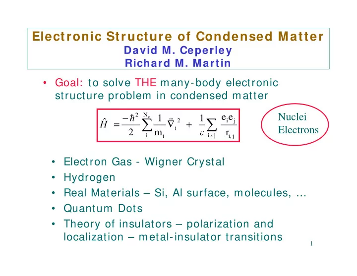
Electronic Structure of Condensed Matter
David M. Ceperley Richard M. Martin
- Electron Gas - Wigner Crystal
- Hydrogen
- Real Materials – Si, Al surface, molecules, …
- Quantum Dots
- Theory of insulators – polarization and
localization – metal-insulator transitions
- Goal: to solve THE many-body electronic
structure problem in condensed matter
∑ ∑
≠
+ ∇ − =
j i j i, j i N i 2 i i 2
r e e 1 m 1 2 ˆ
e