
SLIDE 1
1
- Dynamic Bayesian Networks
Beyond 10708
Graphical Models – 10708 Carlos Guestrin Carnegie Mellon University December 1st, 2006
Readings: K&F: 18.1, 18.2, 18.3, 18.4
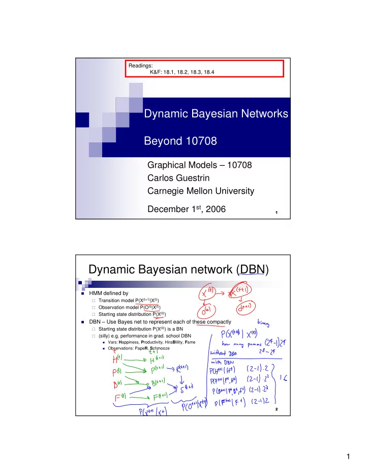
- Dynamic Bayesian network (DBN)
- HMM defined by
Transition model P(X(t+1)|X(t)) Observation model P(O(t)|X(t)) Starting state distribution P(X(0))
- DBN – Use Bayes net to represent each of these compactly
Starting state distribution P(X(0)) is a BN (silly) e.g, performance in grad. school DBN
- Vars: Happiness, Productivity, HiraBlility, Fame
- Observations: PapeR, Schmooze