Bayesian networks (2) Lirong Xia Last class Bayesian networks - PowerPoint PPT Presentation

Bayesian networks (2) Lirong Xia

Last class • Bayesian networks – compact, graphical representation of a joint probability distribution – conditional independence 2

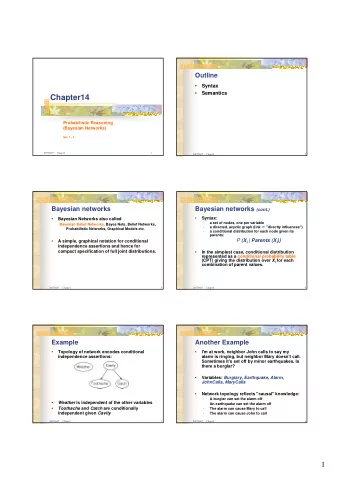
Bayesian network • Definition of Bayesian network (Bayes’ net or BN) • A set of nodes, one per variable X • A directed, acyclic graph • A conditional distribution for each node – A collection of distributions over X, one for each combination of parents’ values ( ) p(X| a 1 ,…, a n ) p X A 1 … A n – CPT: conditional probability table – Description of a noisy “causal” process A Bayesian network = Topology (graph) + Local Conditional Probabilities 3

Probabilities in BNs • Bayesian networks implicitly encode joint distributions – As a product of local conditional distributions n ( ) ( ) = ( ) p x 1 , x 2 ,  x n ∏ p x i parents X i i = 1 – Example: ( ) p +Cavity, +Catch, -Toothache • This lets us reconstruct any entry of the full joint • Not every BN can represent every joint distribution – The topology enforces certain conditional independencies 4

Reachability (D-Separation) • Question: are X and Y conditionally independent given evidence vars {Z}? – Yes, if X and Y “separated” by Z – Look for active paths from X to Y – No active paths = independence! • A path is active if each triple is active: A B C – Causal chain where B is → → unobserved (either direction) A B C – Common cause where B ← → is unobserved A B C – Common effect where B → ← or one of its descendents is observed • All it takes to block a path is a single inactive segment 5

Checking conditional independence from BN graph • Given random variables Z 1 ,…Z p , we are asked whether X ⊥ Y|Z 1 ,…Z p • Step 1: shade Z 1 ,…Z p • Step 2: for each undirected path from X to Y – if all triples are active, then X and Y are NOT conditionally independent • If all paths have been checked and none of them is active, then X ⊥ Y|Z 1 ,…Z p 6

Example R B ⊥ Yes! R B T ⊥ R B T ' ⊥ 7

Example L T T ' Yes! ⊥ L B Yes! ⊥ L B T ⊥ L B T ' ⊥ L B T R , Yes! ⊥ 8

Example • Variables: – R: Raining – T: Traffic – D: Roof drips – S: I am sad • Questions: T D ⊥ T D R Yes! ⊥ T D R S , ⊥ 9

Today: Inference---variable elimination (dynamic programming) 10

Inference • Inference: calculating some useful quantity from a joint probability distribution • Examples: – Posterior probability: ( ) p Q E 1 = e 1 ,  E k = e k – Most likely explanation: ( ) argmax q p Q = q E 1 = e 1 ,  11

Inference • Given unlimited time, inference in BNs is easy • Recipe: – State the marginal probabilities you need – Figure out ALL the atomic probabilities you need – Calculate and combine them • Example: p b , j , m ( ) + + + ( ) p b j , m + + + = p j , m ( ) + + 12

Example: Enumeration • In this simple method, we only need the BN to synthesize the joint entries p b , j , m ( ) + + + = ) ( ) ( ) ( ) p b p e p a b , e p j a p m a ( ) ( + + + + + + + + + + ) ( ) ( ) ( ) p b p e p a b , e p j a p m a ( ) ( + + − + + + − + − + ) ( ) ( ) ( ) p b p e p a b , e p j a p m a ( ) ( + − + + − + + + + + ) ( ) ( ) ( ) p b p e p a b , e p j a p m a ( ) ( + − − + − + − + − 13

Inference by Enumeration? 14

More elaborate rain and sprinklers example Sprinklers p(+R) = .2 Rained were on p(+S) = .6 p(+G|+R,+S) = .9 Neighbor p(+G|+R,-S) = .7 Grass wet walked dog p(+G|-R,+S) = .8 p(+G|-R,-S) = .2 p(+N|+R) = .3 p(+D|+N,+G) = .9 p(+N|-R) = .4 p(+D|+N,-G) = .4 Dog wet p(+D|-N,+G) = .5 p(+D|-N,-G) = .3

Inference Sprinklers p(+R) = .2 Rained were on p(+S) = .6 p(+G|+R,+S) = .9 Neighbor p(+G|+R,-S) = .7 Grass wet walked dog p(+G|-R,+S) = .8 p(+G|-R,-S) = .2 p(+N|+R) = .3 p(+D|+N,+G) = .9 p(+N|-R) = .4 p(+D|+N,-G) = .4 Dog wet p(+D|-N,+G) = .5 p(+D|-N,-G) = .3 • Want to know: p(+R|+D) = p(+R,+D)/P(+D) • Let’s compute p(+R,+D)

Inference Sprinklers p(+R) = .2 Rained were on p(+S) = .6 p(+G|+R,+S) = .9 Neighbor p(+G|+R,-S) = .7 Grass wet walked dog p(+G|-R,+S) = .8 p(+G|-R,-S) = .2 p(+N|+R) = .3 p(+D|+N,+G) = .9 p(+N|-R) = .4 p(+D|+N,-G) = .4 Dog wet p(+D|-N,+G) = .5 p(+D|-N,-G) = .3 • p(+R,+D)= Σ s Σ g Σ n p(+R)p(s)p(n|+R)p(g|+R,s)p(+D|n,g) = p(+R)Σ s p(s)Σ g p(g|+R,s)Σ n p(n|+R)p(+D|n,g)

The formula p(+R,+D)= p(+R)Σ s p(s) Σ g p(g|+R,s) Σ n p(n|+R)p(+D|n,g) f 2 (s,g) f 1 (s) • Order: s>g>n • is what we want to compute • only involves s • only involves s, g 18

Variable elimination Sprinklers p(+R) = .2 Rained were on p(+S) = .6 p(+G|+R,+S) = .9 Neighbor p(+G|+R,-S) = .7 Grass wet walked dog p(+G|-R,+S) = .8 p(+G|-R,-S) = .2 p(+N|+R) = .3 p(+D|+N,+G) = .9 p(+N|-R) = .4 p(+D|+N,-G) = .4 Dog wet p(+D|-N,+G) = .5 p(+D|-N,-G) = .3 • From the factor Σ n p(n|+R)p(+D|n,g) we sum out n to obtain a factor only depending on g • f 2 (s, g) happens to be insensitive to s, lucky! • f 2 (s,+G) = [Σ n p(n|+R)p(+D|n,+G)] = p(+N|+R)P(+D|+N,+G) + p(-N|+R)p(+D|-N,+G) = .3*.9+.7*.5 = .62 • f 2 (s,-G) = [Σ n p(n|+R)p(+D|n,-G)] = p(+N|+R)p(+D|+N,-G) + p(-N|+R)p(+D|-N,-G) = .3*.4+.7*.3 = .33

Calculating f 1 (s) • f 1 (s) = p(+G|+R,s) f 2 (s,+G) + p(-G|+R,s) f 2 (s,-G) • f 1 (+S) = p(+G|+R,+S) f 2 (+S,+G) + p(- G|+R, +S) f 2 (+S,-G) = 0.9*0.62+0.1*0.33=0.591 • f 1 (-S) = p(+G|+R,-S) f 2 (-S,+G) + p(-G|+R, -S) f 2 (-S,-G) = 0.7*0.62+0.3*0.33=0.533 20

Calculating p(+R,+D) • p(+R,+D)= p(+R)p(+S) f 1 (+S) + p(+R)p(- S) f 1 (-S) =0.2*(0.6*0.591+0.4*0.533)=0.11356 21

Elimination order matters Sprinklers p(+R) = .2 Rained were on p(+S) = .6 p(+G|+R,+S) = .9 Neighbor p(+G|+R,-S) = .7 Grass wet walked dog p(+G|-R,+S) = .8 p(+G|-R,-S) = .2 p(+N|+R) = .3 p(+D|+N,+G) = .9 p(+N|-R) = .4 p(+D|+N,-G) = .4 Dog wet p(+D|-N,+G) = .5 p(+D|-N,-G) = .3 • p(+R,+D)= Σ n Σ s Σ g p(+r)p(s)p(n|+R)p(g|+r,s)p(+D|n,g) = p(+R)Σ n p(n|+R)Σ s p(s)Σ g p(g|+R,s)p(+D|n,g) • Last factor will depend on two variables in this case!

General method for variable elimination • Compute a marginal probability p( x 1 ,…, x p ) in a Bayesian network – Let Y 1 ,…,Y k denote the remaining variables – Step 1: fix an order over the Y’s (wlog Y 1 >…>Y k ) – Step 2: rewrite the summation as sth only sth only sth only sth only involving Y 1 , Σ y 1 Σ y 2 …Σ y k -1 Σ y k anything involving involving Y 1 involving Y 1 , Y 2 ,…,Y k -1 Y 2 and X’s X’s and X’s and X’s – Step 3: variable elimination from right to left 23