Distilling Effective Supervision from Severe Label Noise Zizhao - - PDF document

SLIDE 1

Distilling Effective Supervision from Severe Label Noise

Zizhao Zhang, Han Zhang, Sercan Ö. Arık, Honglak Lee, Tomas Pfister Google Cloud AI, Google Brain Abstract

Collecting large-scale data with clean labels for super- vised training of neural networks is practically challenging. Although noisy labels are usually cheap to acquire, existing methods suffer a lot from label noise. This paper targets at the challenge of robust training at high label noise regimes. The key insight to achieve this goal is to wisely leverage a small trusted set to estimate exemplar weights and pseudo labels for noisy data in order to reuse them for supervised

• training. We present a holistic framework to train deep neu-

ral networks in a way that is highly invulnerable to label

• noise. Our method sets the new state of the art on vari-
• us types of label noise and achieves excellent performance
• n large-scale datasets with real-world label noise. For in-

stance, on CIFAR100 with a 40% uniform noise ratio and

• nly 10 trusted labeled data per class, our method achieves

80.2±0.3% classification accuracy, where the error rate is

• nly 1.4% higher than a neural network trained without la-

bel noise. Moreover, increasing the noise ratio to 80%, our method still maintains a high accuracy of 75.5±0.2%, com- pared to the previous best accuracy 48.2%1.

• 1. Introduction

Training deep neural networks usually requires large- scale labeled data. However, the process of data labeling by humans is challenging and expensive in practice, espe- cially in domains where expert annotators are needed such as medical imaging. Noisy labels are much cheaper to ac- quire (e.g., by crowd-sourcing, web search, etc.). Thus, a great number of methods have been proposed to improve neural network training from datasets with noisy labels to take advantage of the cheap labeling practices [48]. How- ever, deep neural networks have high capacity for memo-

• rization. When noisy labels become prominent, deep neural

networks inevitably overfit noisy labeled data [46, 37]. To overcome this problem, we argue that building the dataset wisely is necessary. Most methods consider the set- ting where the entire training dataset is acquired with the

1Source

code available: https://github.com/ google-research/google-research/tree/master/ieg

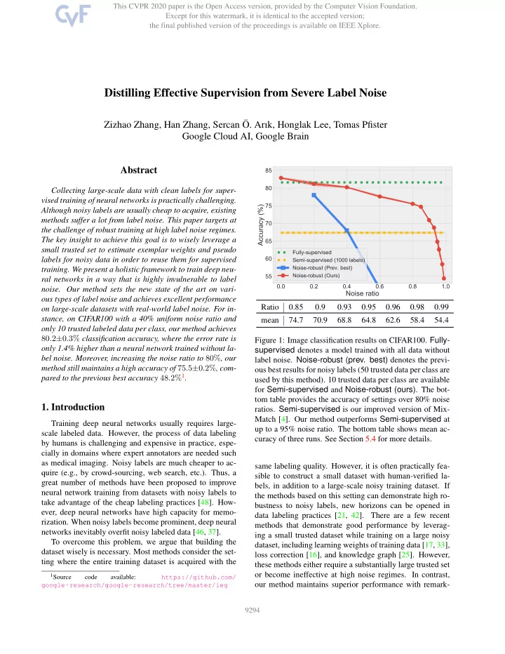
0.0 0.2 0.4 0.6 0.8 1.0

Noise ratio

55 60 65 70 75 80 85

Accuracy (%)

Fully-supervised Semi-supervised (1000 labels) Noise-robust (Prev. best) Noise-robust (Ours)

Ratio 0.85 0.9 0.93 0.95 0.96 0.98 0.99 mean 74.7 70.9 68.8 64.8 62.6 58.4 54.4 Figure 1: Image classification results on CIFAR100. Fully- supervised denotes a model trained with all data without label noise. Noise-robust (prev. best) denotes the previ-

• us best results for noisy labels (50 trusted data per class are

used by this method). 10 trusted data per class are available for Semi-supervised and Noise-robust (ours). The bot- tom table provides the accuracy of settings over 80% noise

• ratios. Semi-supervised is our improved version of Mix-

Match [4]. Our method outperforms Semi-supervised at up to a 95% noise ratio. The bottom table shows mean ac- curacy of three runs. See Section 5.4 for more details. same labeling quality. However, it is often practically fea- sible to construct a small dataset with human-verified la- bels, in addition to a large-scale noisy training dataset. If the methods based on this setting can demonstrate high ro- bustness to noisy labels, new horizons can be opened in data labeling practices [21, 42]. There are a few recent methods that demonstrate good performance by leverag- ing a small trusted dataset while training on a large noisy dataset, including learning weights of training data [17, 33], loss correction [16], and knowledge graph [25]. However, these methods either require a substantially large trusted set

• r become ineffective at high noise regimes. In contrast,
• ur method maintains superior performance with remark-

1

9294

SLIDE 2

ably smaller size of the trusted set (e.g., the previous best method [17] uses up to 10% of the total training data while

• ur method achieves superior results with as low as 0.2%).

Given a small trusted dataset and large noisy dataset, there are two common machine learning approaches to train neural networks. The first is noise-robust training, which needs to handle label noise effects as well as distill correct supervision from the large noisy dataset. Considering the possible harmful effects from label noise, the second ap- proach is semi-supervised learning, which discards noisy labels and treats the noisy dataset as a large-scale unlabeled

• dataset. In Figure 1, we compare methods of the two direc-

tions under such setting. We can observe that the advanced noise-robust method is inferior to semi-supervised meth-

• ds even with a 50% noise ratio (i.e., they cannot utilize

the many correct labels from the other data), motivating the necessity for further investigation of noise-robust training. This also raises a practically interesting question: Should we discard noisy labels and opt in semi-supervised training at high noise regimes for model deployment? Contributions: In response to this question, we propose a highly effective method for noise-robust training. Our method wisely takes advantage of a small trusted dataset to optimize exemplar weights and labels of mislabeled data in order to distill effective supervision from them for su- pervised training. To this end, we generalize a meta re- weighting framework and propose a new meta re-labeling extension, which incorporates conventional pseudo labeling into meta optimization. We further utilize the probe data as anchors to reconstruct the entire noisy dataset using learned data weights and labels and thereby perform supervised

• training. Comprehensive experiments show that even with

extremely noisy labels, our method demonstrates greatly su- perior robustness compared to previous methods (Figure 1). Furthermore, our method is designed to be model-agnostic and generalizable to a variety of label noise types as val- idated in experiments. Our method sets new state of the art on CIFAR10 and CIFAR100 by a significant margin and achieves excellent performance on the large-scale WebVi- sion, Clothing1M, and Food101N datasets with real-world label noise.

• 2. Related Work

In supervised training, overcoming noisy labels is a long- term problem [12, 41, 23, 28, 44], especially important in deep learning. Our method is related to the following dis- cussed methods and directions. Re-weighting training data has been shown to be effec- tive [26]. However, estimating effective weights is chal- lenging. [33] proposes a meta learning approach to di- rectly optimize the weights in pursuit of best validation per-

• formance. [17] alternatively uses teach-student curriculum

learning to weigh data. [13] uses two neural networks to co- train and feed data to each other selectively. [1] models per sample loss and corrects the loss weights. Another direction is modeling confusion matrix for loss correction, which has been widely studied in [36, 29, 38, 30, 1]. For example, [16] shows that using a set of trusted data to estimate the confusion matrix has significant gains. The approach of estimating pseudo labels of noisy sam- ples is another direction and has a close relationship with semi-supervised learning [25, 37, 39, 14, 19, 35, 31]. Along this direction, [32] uses bootstrapping to generate new labels. [23] leverages the popular MAML meta frame- work [11] to verify all label candidates before actual train-

• ing. Besides pseudo labels, building connections to semi-

supervised learning has been recently studied [18]. For ex- ample, [15] proposes to use mixup to directly connect noisy and clean data, which demonstrates the importance of regu- larization for robust training. [15, 1] uses mixup [47] to aug- ment data and demonstrates clear benefits. [10, 18] identi- fies mislabeled data first and then conducts semi-supervised training.

• 3. Background

Reducing the loss weight of mislabeled data has been shown effective in noise-robust training. Here we briefly in- troduce a meta learning based re-weighting (L2R) method [33], serving as a base for the proposed method. L2R is a re- weighting framework that optimizes the data weights in or- der to minimize the loss of an unbiased trusted set matching the test data. The formulation can be briefly summarized as following. Given a dataset of N inputs with noisy labels Du = {(xi, yi), 1 < i < N} and also a small dataset of M of samples with trusted labels Dp = {(xi, yi), 1 < i < M} (i.e., probe data), where M ≪ N. The objective function of training neural networks can be represented as a weighted cross-entropy loss: Θ∗(ω) = arg min

Θ N

• i=1

ωiL(yi, Φ(xi; Θ)), (1) where ω is a vector that its element ωi gives the weight for the loss of one training sample. Φ(·; Θ) is the targeting neu- ral network (with parameters Θ) that outputs the class prob- ability and L(yi, Φ(xi; Θ)) is the standard softmax cross- entropy loss for each training data pair (xi, yi). We omit Θ in Φ(xi; Θ) frequently for conciseness. The above is a standard weighted supervised training

• loss. L2R converts ω as learnable parameters, and formu-

lates a meta learning task to learn optimal ω for each train- ing data in Du, such that the trained model using Equa- tion (1) can minimize the error on a small and trusted dataset Dp [33], measured by the cross-entropy loss Lp

9295

SLIDE 3

• n Dp.

The problem can be solved by repeatedly find- ing a combination of ω that the trained model performs best. However, it is computationally infeasible to com- pute since each update step of it requires training the model until converge before measuring Lp. In practice, it is possible to use an online approximation [33, 11] to perform a single meta gradient-descent step Θt+1(ω) = Θt−α∇Θ N

i ωiL

• yi, Φ(x; Θt)
• , where α is the step size.

Therefore, the meta optimization of ω is defined as ω∗

t = arg min ω,ω≥0

1 M

M

• i

Lp yi, Φ(xi; Θt+1(ω))

• ,

s.t.

• j

ωt,j = 1. (2) The re-weighting coefficients can be obtained by gradient descent ω∗ ≈ ω0 − ∇ωLp|ω=ω0 and then normalization to satisfy the constraints of ω in Equation (2). The method expects that the optimized ω∗ coefficients should assign low weight values to mislabeled data to isolate mislabeled data from clean data. Note that since Θt+1(ω) is a function of ω, the optimization of ω using Lp requires second-order back- propagation (sometimes called gradient-by-gradient) [33].

• 4. Proposed Method

Besides estimating exemplar weights from the noisy data, it is also important to estimate the correct labels via re-labeling process. We informally call this process as es- timation of “Data Coefficients” (i.e., exemplar weights and true labels), which are two major information for construct- ing supervised training. We present a generalized frame- work to estimate data coefficients via meta optimization. The motivation of studying re-labeling is straightfor-

• ward. When the noise ratio is high, a significant amount
• f data would be discarded and thereby would make no

contribution to the model training. To address this ineffi- ciency, it is necessary to enable the reuse of mislabeled data to improve performance at high noise regimes. Different from pseudo labeling in semi-supervised learning [19], a portion of labels in noisy datasets are correct. Thus, distill- ing them effectively bring extra benefits. In contrast to pre- vious pseudo labeling noise-robust methods [23], our pro- posed method constructs a differentiable pseudo re-labeling

• bjective to select the best choice efficiently.

4.1. Initial pseudo label estimator

Utilizing the pseudo labels for unlabeled training data is widely studied for semi-supervised learning [19, 37, 19]. Pseudo labels are usually inferred by the model predictions. Neural networks can be unstable to input augmentations [49, 2]. To generate more robust label guessing, a recent semi-supervised learning method [4] considers averaging predictions over K augmentations. We adopt this simple technique to initialize soft pseudo labels, which is given by averaging predictions of different input augmentations: g(x, Φ)i = Pr

1 τ

i /

• j

Pr

1 τ

j ,

where Pr = 1 K

• Φ(x) +

K−1

• k=1

Φ(ˆ xk)

• (3)

where ˆ xk is k-th random augmentations of input x. g(x) is the estimated pseudo label of x, where gi represents the i-th class probability. τ is a softmax temperature scaling factor used to sharpen the pseudo label distribution (τ = 0.5 in this paper).

4.2. Improved pseudo label initialization

To make pseudo labels effective for supervised training eventually, the distribution of pseudo labels needs to be sharp and consistent across augmented versions of inputs. If the predictions of input augmentations are inconsistent to each other, averaging them with Equation (3) would cause their contributions to cancel out, yielding a flattened pseudo label distribution. From this insight, reducing the inconsis- tency of predictions of augmentations is necessary. There- fore, we propose to improve pseudo label estimation by in- corporating a KL-divergence loss min

Θ

LKL = 1 N

N

• i

KL

• Φ(xi; Θ)
• Φ(ˆ

xi; Θ)

• ,

(4) which penalizes inconsistency of arbitrary input augmenta- tions ˆ xi of xi. The effectiveness of this loss is studied in experiments.

4.3. Meta re-labeling

For each training data x, we now have initial pseudo la- bel g(x, Φ) and its original label y. We formulate the prob- lem of re-labeling as finding the best selection of the two candidates for each data efficiently to reduce the error of the probe data most. Based on the meta re-weighting idea [33], we propose a new objective that combines the estimation of data coefficients efficiently: Θ∗(ω, λ) = arg min

Θ N

• i=1

ωiL

• P(λi), Φ(xi; Θ)
• ,

P(λi) = λiyi + (1 − λi)g(xi, Φ) s.t. 0 ≤ λi ≤ 1, (5) where P is a function of parameter λi that is differentiable. In the meta step, λi is designed to aggregate the original labels and the pseudo labels, which simplifies the back- propagation. Similar to how re-weighting works with second-order back-propagation, we can back-propagate the model using

9296

SLIDE 4

the loss Lp on the probe data to optimize re-labeling coef- ficients λ∗

i . In our implementation, we calculate the sign of

its gradient for each data xi and rectify it: λ∗

i =

• sign
• −

∂ ∂λi E

• Lp|λ=λ0,ω=ω0
• +

. (6) The motivation to use the (rectified) sign of the gradient in- stead of λ ≈ λ0 − ∇λLp|λ=λ0 (as how ω∗ is calculated) are two folds: 1) ∇λLp would become very small at later learning stage when pseudo labels are close to real labels (see Appendix A for mathematical illustration) and 2) sim- ply aggregating yi and g(xi, Φ) using scalar (λ0 − ∇λLp) would make resulting pseudo label distribution not suffi- ciently sharp for supervised training. Therefore, our method proposes to obtain the final pseudo labels as y∗

i =

• yi,

if λ∗

i > 0

g(xi, Φ),

• therwise

(7) After the meta step, we add two cross-entropy losses with respective to optimal ω∗

i and y∗ i ,

Lω∗ =

N

• i

ω∗

i L

• P(λ0), Φ(xi; Θ)
• ,

Lλ∗ =

N

• i

ω0L

• y∗

i , Φ(xi; Θ)

• ,

(8) Similar to L2R, we use momentum SGD for model train-

• ing. L2R sets ω0 = 0 and uses naive gradient descent to

estimate perturbation around ω. In contrast, we compute the meta step model parameters Θt+1 by calculating the ex- act momentum update direction using momentum states of the SGD optimizer2.

4.4. Supervised training

Given estimated data coefficients using probe data, we further leverage the effectiveness of it to construct super- vised training. When introducing probe data for supervised training, appropriate regularizations are important to pre- vent overfitting on the probe data and the consequent fail- ure of meta optimization (i.e., when Lp in Equation (6) gets very small). We divide the data as either possibly-mislabeled (which are assigned with pseudo labels) or possibly-clean (which are assigned with original labels) using the binary criterion I(ωi < T), where T is a scalar threshold. We treat the probe data as anchors to pair each training data and apply mixup [47]. In this way, the model never sees the origi- nal probe data directly but the interpolated point between

2For each training batch, we set initial the values as ω0 = 1/B (where

B is the batch size), treating each data equally. We use λ0 = 0.9 (lean to

• riginal labels) based on the observation of better performance.

Algorithm 1: A training step of our method at time step t Input: Current model parameters Θt, A batch of training data Xu from Du, a batch of probe data Xp from Dp, loss weight k and p, threshold T Output: Updated model parameters Θt+1

1 Generate the augmentation ˆ

Xu of Xu.

2 Estimate the pseudo labels via

g(xu, Φ), xu ∼ Xu∪ ˆ Xu (Section 4.1 & 4.2).

3 Compute optimal data coefficients λ∗ and ω∗ via the

meta step (Section 4.3).

4 Split the training batch Xu (also corresponding ˆ

Xu) to possible clean batch Xc

u and possible mislabeled

batch Xu

u using the binary criterion I(ω∗ < T). 5 Construct the joint batch set (Section 4.4),

Xp ∪ Xu

u ∪ Xc u ∪ ˆ

Xu

u ∪ ˆ

Xc

u,

where ˆ Xu

u ∪ Xu u uses pseudo labels estimated by

g(·, Φ).

6 Compute the total loss for model update

Lω∗ + Lλ∗ + Lp

β + p Lu β + k LKL. 7 Conduct one step stochastic gradient descent to

• btain Θt+1.

probe and training data, which can reduce overfitting on the probe data. In detail, we construct supervised cross-entropy losses on the mixed data in the form of convex combina- tions using the data and their labels given a mixup factor β: Mixβ(a, b) = βa + (1 − β)b, β ∼ Beta(0.5, 0.5). In detail, for each data xa in the concatenated data pool in Dp ∪ ˆ Du ∪Du, we apply pairwise mixup between the input batch and its random permutation, xβ = Mixβ(xa, xb), yβ = Mixβ(ya, yb), where {(xa, ya), (xb, yb) ∈ Dp ∪ ˆ Du ∪ Du}, (9) where ˆ Du is the augmented copy of Du (which is used by Equation (3)). In detail, we introduce two softmax cross- entropy losses: Lp

β for resulting mixed data when xa ∼ Dp

is from probe data and Lu

β when xa ∼ ˆ

Du ∪ Du. The experiments show that our approach can reduce the probe data size to one sample per class.

4.5. End-to-end training process

Our training approach is end-to-end in one stage. A sin- gle gradient descent step can be structured in three sub- steps, meta-optimize data coefficients, construct augmented

9297

SLIDE 5

Table 1: Validation accuracy on CIFAR10 with uniform noise. M denotes the number of trusted (probe) data used. 0.01k indicates 1 image per class. For reference, vanilla training of WRN28-10/ResNet29 leads to 96.1%/92.7% accuracy.

∗

indicates results trained by us. Method M Noise ratio 0.2 0.4 0.8 GCE [48]

• 93.5

89.9±0.2 87.1±0.2 67.9±0.6 MentorNet DD [17] 5k 96.0 92.0 89.0 49.0 RoG [20]

• 94.2

87.4 81.8

• L2R [33]

1k 96.1 90.0±0.4∗ 86.9±0.2 73.0±0.8∗ Arazo et al. [1]

• 93.6

94.0 92.0 86.8 Ours-RN29 0.1k 94.4 92.9±0.2 92.5±0.5 85.6+1.1 Ours 0.01k 96.8 95.4±0.6 94.5±1.0 87.9±5.1 Ours 0.05k 96.8 96.4±0.0 95.5±0.6 91.8±3.0 Ours 0.1k 96.8 96.2±0.2 95.9±0.2 93.7±0.5 Table 2: Validation accuracy on CIFAR100 with uniform noise. Standard training of WRN28-10/RN29 leads to 81.6%/71.3%

• accuracy. 0.1k indicates 1 image per class. ∗ indicates results trained by us.

Method M Noise ratio 0.2 0.4 0.8 GCE [48]

• 81.4

66.8±0.4 61.8±0.2 47.7±0.7 MentorNet [17] 5k 79.0 73.0 68.0 35.0 L2R [33] 1k 81.2 67.1±0.1∗ 61.3+2.0 35.1±1.2∗ Arazo et al. [1] 70.3 68.7 61.7 48.2 Ours-RN29 1k 72.1 69.3±0.5 67.0±0.8 60.7±1.0 Ours 0.1k 83.0 77.4±0.4 75.1±1.1 62.1±1.2 Ours 0.5k 83.0 80.4±0.5 79.6±0.3 73.6±1.5 Ours 1k 83.0 81.2±0.7 80.2±0.3 75.5±0.2 Table 3: Asymmetric noise on CIFAR10. Method Noise ratio 0.2 0.4 0.8 GCE [48] 89.5±0.3 82.3±0.7

• LC [30]

89.1±0.5 83.6±0.3

• Ours-RN29

92.7±0.2 90.2±0.5 78.9±3.5 Ours 96.5±0.2 94.9±0.1 79.3±2.4 data, and update the model using aggregated losses. Al- gorithm 1 illustrates a complete training step and specifies the joint objectives and their coefficients. Appendix B dis- cusses the training efficiency.

• 5. Experiments

5.1. Implementation details and experimental setup

Here we discuss training details and hyperparameters that are shown to be useful for our experiments. More train- ing details can be found in the Appendix. Model training: We adopt the Cosine learning rate de- Table 4: Experiments with semantic noise where labels are generated by a neural network trained on limited data. The resulting noise ratio is shown in parentheses. Method CIFAR10 (34%) CIFAR100 (37%) RoG [20] 70.0 53.6 L2R∗ [33] 71.0 56.9 Ours-RN29 81.8 65.1 Ours 88.3 73.7 cay with warm restarting [27]3. In detail, we selected mod- els at the lowest learning rate before the end of scheduled epochs for reporting result. We observe 3%-5% accuracy improvement on CIFAR datasets compared with the stan- dard learning rate decay schedule (i.e., as used by L2R [33]), especially at large noise ratios. Figure 2 compares the

3This learning rate schedule restarts from a larger value after each “co-

sine” cycle, so it yields a training curve with repeated ‘jag’ shapes (see Figure 2). We set the initial cycle length to be one epoch, and after then cycle length increases by a factor of 1.5 and meanwhile the restart learning rate decreases by a factor of 0.9 as described in [27].

9298

SLIDE 6

10000 20000 30000 40000 50000 60000 70000 80000 90000

Steps

10 20 30 40 50 60 70 80

Accuracy (%) Standard decay Cosine decay

Figure 2: Comparison with standard learning rate decay

• strategy. We use the commonly accepted setting (also used

by L2R): the initial learning rate is 0.1, the learning rate de- cays to previous 0.1x at 40K and 50K steps. We show the training curves on CIFAR10 with 40% uniform label noise. Dotted and solid lines are evaluation and training accuracy curves, respectively. training curves. Although it works particularly well in our method, we do not observe strong benefit for either training vanilla neural networks or training L2R. Further investiga- tion are left as future work. Augmentation: Augmentation generates pixel-level perturbations on the original training inputs, which plays a critical role in Equation (3) and (4). We use the recently-proposed data augmentation technique based on policy-based augmentation (PA), AutoAugment [6], in

• ur experiments.

PA includes data processes of (policy augmentation→flip→random crop→cutout [9]). In detail, for each input image, we first generate one standard aug- mentation (random crop and horizontal flip) and then apply PA to generate K random augmentations on top of the stan- dard one. We fix K = 2 augmentations in our experiments. We further analyze the effects of learned policies and ran- dom policies (i.e., with no learning required) in Section 6.

5.2. CIFAR noisy label experiments

We follow [33, 17] to conduct CIFAR10 and CIFAR100 experiments. For all CIFAR experiments with different noise types and ratios, we set T = 1, p = 5, k = 20, which are empirically determined on CIFAR10 with 40% uniform noise. Standard deviation are obtained over 3 runs with random seeds (and random data splits). We compare the proposed method against several recent methods, which have achieved leading performance on public benchmarks. Similar to L2R, we use the Wide ResNet (WRN28-10) [45] as default, unless specified otherwise for fair comparison. We also test our method using ResNet29 (RN29)4, which is much smaller than the ones used by compared methods. Common random label noise: Table 1 compares the results for CIFAR10 with uniform noise ratios of 0.2, 0.4,

4We follow this v2 implementation https://github.com/

keras-team/keras/blob/master/examples/cifar10_ resnet.py, which contains 0.84M parameters.

and 0.8. Our method yields 96.5% accuracy at 20% noise ratio and 94.7% accuracy at 80% noise ratio, demonstrat- ing nearly noise-invulnerable performance. It still achieves the best performance with ResNet29. We also train our full method with 0% noise as reference. Table 2 compares the results in CIFAR100 with uniform noise ratios of 0.2, 0.4, and 0.8. Additionally, we test our method with 10 images, 5 images and the extreme case of 1 image per class as probe

• data. MentorNet uses 5k clean images (50 per class) while
• ur method reduces this number by up to 50x and maintains
• utperformed accuracy.

Semantic label noise: Next, we test our method on more realistic noisy settings on CIFAR. By default, 10 images per class are used as probe data. First, Table 3 compares the re- sults on CIFAR10 with asymmetric noise ratios of 0.2, 0.4, and 0.8. Asymmetric noise is known as a more realistic set- ting because it corrupts semantically-similar classes (e.g., truck and automobile, or bird and airplane) [30]. Second, we follow RoG [20] to generate semantically noisy labels by using a trained VGG-13 [34] on 5% of CIFAR10 and 20% of CIFAR1005. Table 4 reports the compared results. Synthetic open-set noise: Open-set is a unique type

• f noise that occurs in images rather than labels [3, 40].

We test our method on three kinds of synthetic open-set noisy labels provided by [20] in Table 5. In all seman- tic noise settings, our method consistently outperforms the compared methods with a significant margin. From base- line comparison of supervised training in Table 5, we can see model capacity is beneficial for performance. However, L2R, which uses WRN28-10, does not outperform its su- pervised WRN28-10, which implies that data re-weighting might not sufficient to deal with this noise type.

5.3. Large-scale real-world experiments

WebVision [24] is a large-scale dataset which consists

• f real-world noisy labels. It contains 2.4 million images

and shares the 1000 classes of ImageNet [8]. We follow [17] to create a mini version of WebVision, which includes the Google subset images of the top 50 classes. We train all models using the WebVision training set and evaluate

• n the ImageNet validation set. We modify p = 4 and

k = 8 for mini and 0.4 for full. The default architecture is InceptionResNetv2, the same as compared methods. We also test a smaller ResNet-50. To create the probe dataset, we split 10 images per class from the ImageNet training

• data. We only observe slight (<0.5%) gain when we train

InceptionResNetv2/ResNet-50 by adding the probe data in training data. As shown in Table 6, our method significantly

• utperforms compared methods.

Clothing1M [42] and Food101N [22] are another two large-scale datasets with real-world noisy labels. We fol-

5We directly use the data provided by RoG authors. VGG-13 the hard-

est setting.

9299

SLIDE 7

Table 5: Open-set noise on CIFAR10. Each column indicates where the noisy out-of-distribution images are from. RoG uses DenseNet-100 and L2R uses WRN28-10. We run the baseline for better comparison (the first block of the table). Method CIFAR100 CIFAR100+ImageNet ImageNet RN29 77.8 80.3 84.4 DenseNet-100 [20] 79.0 86.7 81.6 WRN28-10 82.8 84.7 88.7 L2R [33] 81.8 81.3 85.0 RoG [20] 83.4 87.1 84.4 Ours-RN29 86.4 87.4 90.0 Ours 92.3 93.0 94.0 Table 6: Large-scale WebVision experiments on mini and full versions. The top-1/top-5 accuracy on the ImageNet validation set are reported. Method mini full Co-teaching [13] 61.5/84.7

• Chen el al. [5]

61.6/85.0

• MentorNet [17]

63.8/85.8 64.2/84.8 Ours-RN50 78.0/94.4 65.8/85.8 Ours 80.0/94.9 69.0/88.3 Table 7: Food101N experiments. Method Accuracy ResNet50 [22] 81.44 CleanNet [22] 83.95 Self-Learning [14] 85.11 Ours-RN50 87.57 low their specific settings and train our method to com- pare with previous methods. Each dataset contains a hu- man verified train subset, which is used as our probe data. We use ResNet50 with random initialization. Image size is

• 224x224. The comparison result of Food101N are shown in

Table 7. Our method achieves 77.21% on the Clothing1M dataset.

5.4. Comparison to semi-supervised learning

We compare our method to one of the advanced semi- supervised learning methods, MixMatch [4], and verify how much useful information our method can distill from misla- beled data. Figure 1 shows the comparisons and Table 8 re- ports the detailed results. Given the same trusted set (probe data), our method largely improves the semi-supervised ac- curacy given 80% label noise ratio on CIFAR100. Addition- ally, the proposed technique (i.e., KL-loss in Section 4.2) improves pseudo labeling so it is supposed to be useful for the compared MixMatch. As shown in Table 8, it is interest- ing to find out that our extension (denoted as MixMath-KL) shows remarkable benefits for semi-supervised learning, for

20000 40000 60000 80000 100000

Steps

10 20 30 40 50 60 70

Accuracy (%)

k = 1 k = 5 k = 20

Figure 3: Training curves on CIFAR100 with uniform 80% label noise under different LKL loss weight k (defined in Algorithm 1). Dotted are solid lines are train and evaluation accuracy curves, respectively. Since the noise ratio is 80%, the average training accuracy is expected to be lower than 20%, otherwise the model starts to overfit. When we use a small k, the model becomes to overfit after 70k iterations. example, it improves accuracy from 34.5% to 57.6%.

• 6. Ablation Studies and Discussions

Here we study the individual objective components and their importance. Table 9 summarizes the ablation study results (referred to as M-#) and we discuss them below. The effects of LKL: Based on our empirical observa- tions, LKL plays an important role in preventing neural net- works from overfitting to samples with wrong labels, espe- cially at extreme noise ratios. M-4 shows results without

• LKL. Figure 3 shows the training curves with different co-

efficient k for LKL. At around 80k iterations, the curve of β = 1 starts to overfit to noisy labels and simultaneously the validation accuracy starts to decrease. β = 20 is much more efficient in overcoming this. The effects of Lβ: M-6 shows the result without Lβ. The performance loss is significant at 80% noise ratio. The intermediate step of Lβ is mixup. It helps the introduc- tion of probe data in supervised training and reduces over- fitting (see Section 4.4). M-9 and M-10 study its effect. If we reduce the probe data size to be 1 sample per class, the accuracy drop becomes significant w/o mixup (the full

9300

SLIDE 8

Table 8: A comparison to semi-supervised methods and our semi-supervised extension (MixMatch-KL). MixMatch and MixMatch-KL∗ use WRN-28-2. 10 labeled data per class are used for semi-supervised training and the probe data of our

• method. Previous best scores for this task are compared.

Semi-supervised Noise-robust (80% noise) Dataset MixMatch [4] MixMatch-KL∗ MixMatch-KL

• Prev. best [1]

Ours CIFAR10 51.2 92.4±0.7 94.5±0.3 86.8 93.7±0.5 CIFAR100 34.5 57.6±0.4 67.3±0.3 48.2 75.2±0.2 Table 9: Ablation study on CIFAR100. /✗ indicates the corresponding component is enabled/disabled. So M-1 is equal to L2R; M-5 (bold) is the full method. Abbreviations are defined in text. M-# Component Noise ratio LKL Lβ PA λ 0.4 0.8 1 64.43 33.52 2

• 66.14

36.04 3

• 67.82

37.01 4

• 78.06

61.81 5

• 79.96

75.42 6 ✗ 73.63 54.76 7 ✗ 79.16 72.69 8 ✗ 81.05 74.04 9 w/o mixup 10 / class 78.4 72.7 10 w/o mixup 1 / class 62.5 47.1 method with 1 sample per class achieves 75.1%/62.1% ac- curacy with 40%/80% noise ratios, as shown in Table 2). The effects of data augmentation: The disadvantage of learned PA as used by our method is that it requires learned policies on CIFAR, implying the use of extra labeled data [43]. We study the contribution of the learned policy to our method with two different experiments. First, M-3 and M-7 show the results without learned policy augmentation (we

• nly use flip → random crop → cutout). The accuracy de-

crease is minor given 40% noise and less than 3% given 80% noises. Second, we completely randomize the policies following [7], we observe that accuracy are almost identi- cal to the original results at all noise ratios. The two ex- periments indicate that our method does not rely on leaned policies and removing them keeps our method effective. The effects of λ: Our proposed meta re-labeling (Equa- tion (5)) is very effective for high noise ratios. We observe comparable performance of models without re-labeling at low noise ratios (e.g. M-5 vs M-8), indicating higher effec- tiveness of meta re-labeling given higher noise ratios, how- ever, less effectiveness at low noise ratios. Figure 4 (top) shows the average λ during the training process (the value

• f noise labels are obtained by peeping ground truth). It

learns to reduce λ for mislabeled data in order to promote

20000 40000 60000 80000

Training steps

0.0 0.2 0.4 0.6 0.8 1.0

Average

Noisy labels Clean labels

0.80 0.85 0.90 0.93 0.95 0.96 0.98 0.99

Noise ratio

40 50 60 70

Accuracy (%)

Ours w/o Ours

Figure 4: Analysis of λ. Top: The average λ of noisy and clean labels on CIFAR10 with 40% noise. The average λ at 50 epoch converts to ∼0.6, indicting 40% mislableled data are detected. Bottom: Accuracy (w/o λ) at extreme noise ratios on CIFAR100. the use of pseudo labels, and vice versa for clean data. Fig- ure 4 (bottom) demonstrates the significant advantage of the proposed λ at extreme noise ratios.

• 7. Conclusion

We present a holistic noise-robust training method to address the challenges of severe label noise. Our ap- proach leverages a small trusted set to estimate the exem- plar weights and labels (namely Data Coefficients) and train models in a supervised manner that is highly invulnerable to label noise. Comprehensive experiments are conducted on datasets with various types of label corruptions. Learning from noisy labels is a highly desirable capabil-

• ity. This paper suggests two takeaways. First, small trusted

set is not costly but highly valuable to acquire. Design- ing noise-robust methods that leverage them can have much higher potential to improve performance. To the best of our knowledge, this paper is the first to demonstrate superior robustness against noise regimes as high as over 90%.

Acknowledgments

We would like to thank Liangliang Cao, Kihyuk Sohn, David Berthelot, Qizhe Xie, and Chen Xing for their valu- able discussions.

9301

SLIDE 9

References

[1] Eric Arazo, Diego Ortego, Paul Albert, Noel E O’Connor, and Kevin McGuinness. Unsupervised label noise modeling and loss correction. ICML, 2019. 2, 5, 8 [2] Aharon Azulay and Yair Weiss. Why do deep convolutional networks generalize so poorly to small image transforma- tions? arXiv preprint arXiv:1805.12177, 2018. 3 [3] Abhijit Bendale and Terrance E Boult. Towards open set deep networks. In Proceedings of the IEEE conference on computer vision and pattern recognition, pages 1563–1572,

• 2016. 6

[4] David Berthelot, Nicholas Carlini, Ian Goodfellow, Nico- las Papernot, Avital Oliver, and Colin Raffel. Mixmatch: A holistic approach to semi-supervised learning. NeurIPS,

• 2019. 1, 3, 7, 8

[5] Pengfei Chen, Benben Liao, Guangyong Chen, and Shengyu

• Zhang. Understanding and utilizing deep neural networks

trained with noisy labels. arXiv preprint arXiv:1905.05040,

• 2019. 7

[6] Ekin D Cubuk, Barret Zoph, Dandelion Mane, Vijay Vasude- van, and Quoc V Le. Autoaugment: Learning augmentation policies from data. CVPR, 2019. 6 [7] Ekin D Cubuk, Barret Zoph, Jonathon Shlens, and Quoc V

• Le. Randaugment: Practical data augmentation with no sep-

arate search. arXiv preprint arXiv:1909.13719, 2019. 8 [8] Jia Deng, Wei Dong, Richard Socher, Li-Jia Li, Kai Li, and Li Fei-Fei. Imagenet: A large-scale hierarchical image

• database. In CVPR. 6

[9] Terrance DeVries and Graham W Taylor. Improved regular- ization of convolutional neural networks with cutout. arXiv preprint arXiv:1708.04552, 2017. 6 [10] Yifan Ding, Liqiang Wang, Deliang Fan, and Boqing Gong. A semi-supervised two-stage approach to learning from noisy labels. In WACV, 2018. 2 [11] Chelsea Finn, Pieter Abbeel, and Sergey Levine. Model- agnostic meta-learning for fast adaptation of deep networks. In ICML, 2017. 2, 3 [12] Benoît Frénay and Michel Verleysen. Classification in the presence of label noise: a survey. IEEE transactions on neu- ral networks and learning systems, 2013. 2 [13] Bo Han, Quanming Yao, Xingrui Yu, Gang Niu, Miao Xu, Weihua Hu, Ivor Tsang, and Masashi Sugiyama. Co- teaching: Robust training of deep neural networks with ex- tremely noisy labels. In NeurIPS, 2018. 2, 7 [14] Jiangfan Han, Ping Luo, and Xiaogang Wang. Deep self- learning from noisy labels. ICCV, 2019. 2, 7 [15] Ryuichiro Hataya and Hideki Nakayama. Unifying semi- supervised and robust learning by mixup. 2019. 2 [16] Dan Hendrycks, Mantas Mazeika, Duncan Wilson, and Kevin Gimpel. Using trusted data to train deep networks

• n labels corrupted by severe noise. In NeurIPS, 2018. 1, 2

[17] Lu Jiang, Zhengyuan Zhou, Thomas Leung, Li-Jia Li, and Li Fei-Fei. Mentornet: Learning data-driven curriculum for very deep neural networks on corrupted labels. ICML, 2018. 1, 2, 5, 6, 7 [18] Youngdong Kim, Junho Yim, Juseung Yun, and Junmo Kim. Nlnl: Negative learning for noisy labels. ICCV, 2019. 2 [19] Dong-Hyun Lee. Pseudo-label: The simple and efficient semi-supervised learning method for deep neural networks. In ICML Workshop, 2013. 2, 3 [20] Kimin Lee, Sukmin Yun, Kibok Lee, Honglak Lee, Bo Li, and Jinwoo Shin. Robust inference via generative classifiers for handling noisy labels. ICML, 2019. 5, 6, 7 [21] Kuang-Huei Lee, Xiaodong He, Lei Zhang, and Linjun

• Yang. Cleannet: Transfer learning for scalable image classi-

fier training with label noise. In CVPR, 2018. 1 [22] Kuang-Huei Lee, Xiaodong He, Lei Zhang, and Linjun

• Yang. Cleannet: Transfer learning for scalable image classi-

fier training with label noise. In CVPR, 2018. 6, 7 [23] Junnan Li, Yongkang Wong, Qi Zhao, and Mohan S Kankan-

• halli. Learning to learn from noisy labeled data. In CVPR,
• 2019. 2, 3

[24] Wen Li, Limin Wang, Wei Li, Eirikur Agustsson, and Luc Van Gool. Webvision database: Visual learning and under- standing from web data. arXiv preprint arXiv:1708.02862,

• 2017. 6

[25] Yuncheng Li, Jianchao Yang, Yale Song, Liangliang Cao, Jiebo Luo, and Li-Jia Li. Learning from noisy labels with

• distillation. In ICCV, 2017. 1, 2

[26] Tongliang Liu and Dacheng Tao. Classification with noisy labels by importance reweighting. Transactions on pattern analysis and machine intelligence (TPAMI), 2015. 2 [27] Ilya Loshchilov and Frank Hutter. Sgdr: Stochastic gradient descent with warm restarts. ICLR, 2017. 5 [28] Xingjun Ma, Yisen Wang, Michael E Houle, Shuo Zhou, Sarah M Erfani, Shu-Tao Xia, Sudanthi Wijewickrema, and James Bailey. Dimensionality-driven learning with noisy la-

• bels. ICML, 2018. 2

[29] Nagarajan Natarajan, Inderjit S Dhillon, Pradeep K Raviku- mar, and Ambuj Tewari. Learning with noisy labels. In NeurIPS, 2013. 2 [30] Giorgio Patrini, Alessandro Rozza, Aditya Krishna Menon, Richard Nock, and Lizhen Qu. Making deep neural networks robust to label noise: A loss correction approach. In CVPR,

• 2017. 2, 5, 6

[31] Hieu Pham, Qizhe Xie, Zihang Dai, and Quoc V Le. Meta pseudo labels. arXiv preprint arXiv:2003.10580, 2020. 2 [32] Scott Reed, Honglak Lee, Dragomir Anguelov, Christian Szegedy, Dumitru Erhan, and Andrew Rabinovich. Train- ing deep neural networks on noisy labels with bootstrapping. CVPR, 2015. 2 [33] Mengye Ren, Wenyuan Zeng, Bin Yang, and Raquel Urta-

• sun. Learning to reweight examples for robust deep learning.

ICML, 2018. 1, 2, 3, 5, 6, 7 [34] Karen Simonyan and Andrew Zisserman. Very deep convo- lutional networks for large-scale image recognition. ICLR,

• 2015. 6

[35] Kihyuk Sohn, David Berthelot, Chun-Liang Li, Zizhao Zhang, Nicholas Carlini, Ekin D Cubuk, Alex Kurakin, Han Zhang, and Colin Raffel. Fixmatch: Simplifying semi- supervised learning with consistency and confidence. arXiv preprint arXiv:2001.07685, 2020. 2 [36] Sainbayar Sukhbaatar, Joan Bruna, Manohar Paluri, Lubomir Bourdev, and Rob Fergus. Training convolutional networks with noisy labels. ICLR, 2015. 2 9302

SLIDE 10

[37] Daiki Tanaka, Daiki Ikami, Toshihiko Yamasaki, and Kiy-

• haru Aizawa.

Joint optimization framework for learning with noisy labels. In CVPR, 2018. 1, 2, 3 [38] Ryutaro Tanno, Ardavan Saeedi, Swami Sankaranarayanan, Daniel C Alexander, and Nathan Silberman. Learning from noisy labels by regularized estimation of annotator confu-

• sion. CVPR, 2019. 2

[39] Andreas Veit, Neil Alldrin, Gal Chechik, Ivan Krasin, Abhi- nav Gupta, and Serge Belongie. Learning from noisy large- scale datasets with minimal supervision. In CVPR, 2017. 2 [40] Yisen Wang, Weiyang Liu, Xingjun Ma, James Bailey, Hongyuan Zha, Le Song, and Shu-Tao Xia. Iterative learning with open-set noisy labels. In CVPR, 2018. 6 [41] Yisen Wang, Xingjun Ma, Zaiyi Chen, Yuan Luo, Jinfeng Yi, and James Bailey. Symmetric cross entropy for robust learning with noisy labels. In ICCV, 2019. 2 [42] Tong Xiao, Tian Xia, Yi Yang, Chang Huang, and Xiaogang

• Wang. Learning from massive noisy labeled data for image
• classification. In CVPR, 2015. 1, 6

[43] Qizhe Xie, Zihang Dai, Eduard H. Hovy, Minh-Thang Lu-

• ng, and Quoc V. Le.

Unsupervised data augmentation. arXiv:1904.12848, 2019. 8 [44] Kun Yi and Jianxin Wu. Probabilistic end-to-end noise cor- rection for learning with noisy labels. CVPR, 2019. 2 [45] Sergey Zagoruyko and Nikos Komodakis. Wide residual net-

• works. BMVC, 2016. 6

[46] Chiyuan Zhang, Samy Bengio, Moritz Hardt, Benjamin Recht, and Oriol Vinyals. Understanding deep learning re- quires rethinking generalization. ICLR, 2017. 1 [47] Hongyi Zhang, Moustapha Cisse, Yann N Dauphin, and David Lopez-Paz. mixup: Beyond empirical risk minimiza-

• tion. ICLR, 2017. 2, 4

[48] Zhilu Zhang and Mert Sabuncu. Generalized cross entropy loss for training deep neural networks with noisy labels. In NeurIPS, 2018. 1, 5 [49] Stephan Zheng, Yang Song, Thomas Leung, and Ian Good-

• fellow. Improving the robustness of deep neural networks

via stability training. In CVPR, 2016. 3 9303