Discrete Probability Distributions Bernoulli with parameter p: - - PowerPoint PPT Presentation

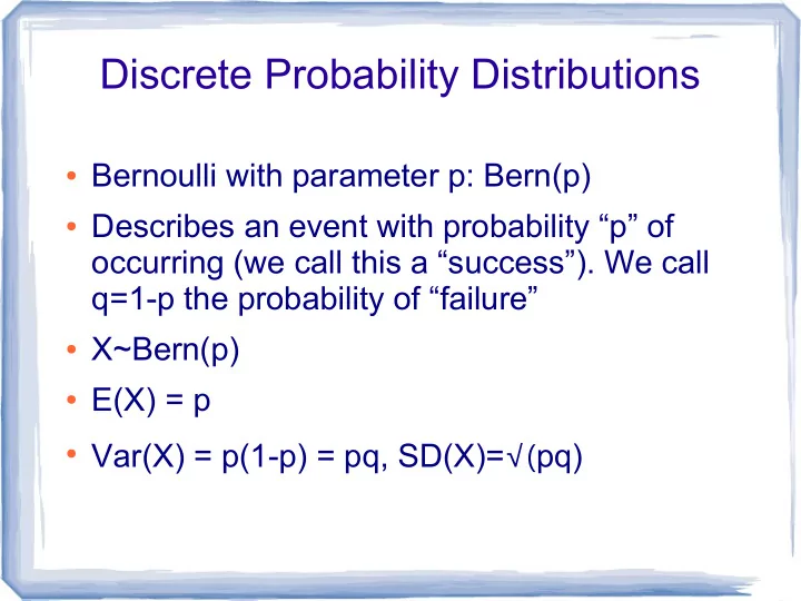
Discrete Probability Distributions

• Bernoulli with parameter p: Bern(p)
• Describes an event with probability “p” of
• ccurring (we call this a “success”). We call

q=1-p the probability of “failure”

• X~Bern(p)
• E(X) = p
• Var(X) = p(1-p) = pq, SD(X)=√(pq)

Bernoulli Example

• You drop your toast and as we all know toast

has a 75% chance of landing butter side-

• down. If it lands butter-side down you need to

buy new toast for $1, but if it's butter side up, the 5 second rule applies and you don't have to buy new toast! What is the expected cost and standard deviation of dropping toast?

• E(X)=p*$1=$.75
• SD(X)=√Var(X)=√(pq)=√.1875≈$.433

Multiple Bernoulli Trials

• When we are performing multiple independent

Bernoulli trials, we make new distributions

• Binomial Distribution: Models the number of

successes obtained from “n” independent Bernoulli trials

• Geometric Distribution: Models the number of

independent Bernoulli trials until (and including) the first success

Binomial Distribution

• X~Binom(n,p) means X follows a Binomial

model of “n” independent trials with probability “p” of success

• P(X=k) is the probability of “k” successes
• P(X=k)=C(n,k)*pk*q(n-k)
• C(n,k) counts all combinations of k out of n

(ie., which of the n trials are the k successes)

Binomial Histogram

• Histogram of Binomial(20, 0.50)

“n choose k”

• C(n,k) is sometimes written
• We say “n choose k”
• The formula is
• The TI-83/84 has this built in.
• Go to [MATH]>[PRB] and choose “nCr”
• eg., “8 nCr 3” = 56. This means there are 56

possible combinations of 3 out of 8 things.

(

n k)

(

n k)= n! k !(n−k)!

Back to the Binomial

• X~Binom(n,p)
• E(X)=np
• Var(X)=npq, SD(X)=√(npq)
• P(X≤k) = P(X=0) + P(X=1) +∙∙∙+ P(X=k)

P( X =k)=( n k) p

k q n−k

Binomial Example

• An archer hits his mark 85% of the time. He

fires 5 arrows. What is the probability that 3 of them hit?

• X~Binom(5,.85) because n=5, p=.85
• E(X)=np=5*.85=4.25
• Var(X)=npq=5(.85)(.15)=.6375
• SD(X)=√Var(X)=√.6375=.7984

P( X =3)=( 5 3)(.85)

3(.15) 2=.13817

Geometric Distribution

• X~Geometric(p) means X follows a Geometric

Model with probability “p” of success

• P(X=k) = p*qk-1
• ie, the probability of 1 success and k-1 failures
• E(X)=1/p
• Var(X)=q/p2, SD(X)=√(q/p2)

Geometric Histogram

• Histogram of Geom(1/3)

Geometric Example

• At the apple factory, a barrel of apples has a

4% chance of being spoiled. Your job is to do quality control. What is the expected number

• f barrels to check until you find a spoiled

barrel? What is the Standard Deviation?

• X~Geometric(.04) so E(X)=1/.04=25
• Var(X)=q/p2=.96/.042=600 so

SD(X)=√600≈24.5

Texas Instruments to the Rescue!

• TI-83/84 make use of the Geometric and

Binomial models much easier

• [2nd][VARS] gives access to:

– 0:binompdf( – A:binomcdf( – D:geometpdf( – E:geometcdf(

How to use TI-83/84 distributions

• binompdf(n,p,k) gives the probability of

exactly k successes out of n trials with probability p

• binomcdf(n,p,k) gives the probability of k
• r fewer successes out of n trials
• geometpdf(p,k) gives the probability that it

takes exactly k trials to get a success

• geometcdf(p,k) gives the probability that it

takes k or fewer trials to get a success