Digital Geometry Processing Basics University of British Columbia - - PDF document

SLIDE 1

Page 1

Basics

Digital Geometry Processing

University of British Columbia 1

Mesh Basics: Definitions, Topology & Data Structures

University of British Columbia 2

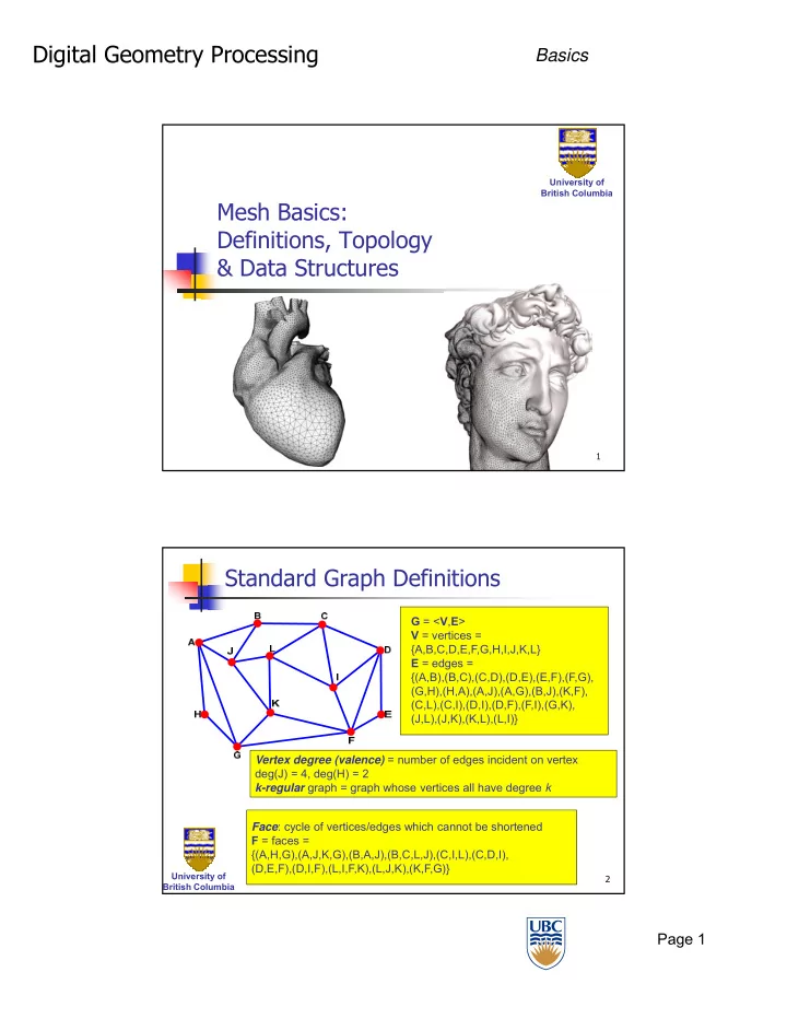
Standard Graph Definitions

G = <V,E> V = vertices = {A,B,C,D,E,F,G,H,I,J,K,L} E = edges = {(A,B),(B,C),(C,D),(D,E),(E,F),(F,G), (G,H),(H,A),(A,J),(A,G),(B,J),(K,F), (C,L),(C,I),(D,I),(D,F),(F,I),(G,K), (J,L),(J,K),(K,L),(L,I)} Vertex degree (valence) = number of edges incident on vertex deg(J) = 4, deg(H) = 2 k-regular graph = graph whose vertices all have degree k Face: cycle of vertices/edges which cannot be shortened F = faces = {(A,H,G),(A,J,K,G),(B,A,J),(B,C,L,J),(C,I,L),(C,D,I), (D,E,F),(D,I,F),(L,I,F,K),(L,J,K),(K,F,G)}

SLIDE 2

Page 2

Basics

Digital Geometry Processing

University of British Columbia 3

Connectivity

Graph is connected if there is a path of edges connecting every two vertices Graph is k-connected if between every two vertices there are k edge-disjoint paths Graph G’=<V’,E’> is a subgraph of graph G=<V,E> if V’ is a subset of V and E’ is the subset of E incident on V’ Connected component of a graph: maximal connected subgraph Subset V’ of V is an independent set in G if the subgraph it induces does not contain any edges of E

University of British Columbia 4

Graph Embedding

if each vertex is

d

in R embedded Graph is

d

assigned a position in R

2

Embedding in R

3

Embedding in R

SLIDE 3

Page 3

Basics

Digital Geometry Processing

University of British Columbia 5

Planar Graphs

Planar Graph Plane Graph Straight Line Plane Graph Planar graph: graph whose vertices and edges can be embedded in R2 such that its edges do not intersect Every planar graph can be drawn as a straight-line plane graph

University of British Columbia 6

Triangulation

Triangulation: straight line plane graph all of whose faces are triangles Delaunay triangulation of a set of points: unique set of triangles such that the circumcircle of any triangle does not contain any other point Delaunay triangulation avoids long and skinny triangles

SLIDE 4

Page 4

Basics

Digital Geometry Processing

University of British Columbia 7

Meshes

Boundary edge: adjacent to exactly one face Regular edge: adjacent to exactly two faces Singular edge: adjacent to more than two faces Closed mesh: mesh with no boundary edges Manifold mesh: mesh with no singular edges Mesh: straight-line graph embedded in R3

Non-Manifold Closed Manifold Open Manifold

Corners  V x F Half-edges  E x F

University of British Columbia 8

Planar Graphs and Meshes

Every manifold mesh is planar !! (almost)

SLIDE 5

Page 5

Basics

Digital Geometry Processing

University of British Columbia 9

Topology

Euler-Poincare Formula v+f-e = 2(c-g)-b

v = # vertices c = # conn. comp f = # faces g = genus e = # edges b = # boundaries

v =12 f = 14 e = 25 c = 1 g = 0 b = 1

Genus of graph: half of maximal number of closed paths that do not disconnect the graph (number of “holes”) Genus(sphere)= 0 Genus(torus) = 1

University of British Columbia 10

Topology Quiz

What can you say about the genus of these meshes ?

SLIDE 6

Page 6

Basics

Digital Geometry Processing

University of British Columbia 11

Exercises

Theorem: In closed manifold mesh: 2e  3f (equality for triangle mesh), 2e  3v Corollary: No closed manifold triangle mesh can have 7 edges Corollary: 2f-4  v Theorem: Average vertex degree in closed manifold triangle mesh is ~6 Proof: In such a mesh, f = 2e/3 By Euler’s formula: v+2e/3-e = 2-2g hence e = 3(v-2+2g) and f = 2(v-2+2g) So Average(deg) = 2e/v = 6(v-2+2g)/v ~ 6 for large v Corollary: Only toroidal (g=1) closed manifold triangle mesh can be regular (all vertex degrees are 6) Proof: In regular mesh average degree is exactly 6 Can happen only if g=1

Does Euler’s theorem imply that any planar graph has an independent set of size at least ¼ n ? University of British Columbia 12

Orientability

Straight line graph is orientable if orientations of its faces can be chosen so that each edge is

• riented in both directions

Orientation of a face is clockwise or anticlockwise

• rder in which its vertices and edges are listed

This defines the direction of face normal

Oriented F={(L,J,B),(B,C,L),(L,C,I), (I,K,L),(L,K,J)} Not Oriented F={(B,J,L),(B,C,L),(L,C,I), (L,I,K),(L,K,J)}

Backface Culled Not Backface Culled

SLIDE 7

Page 7

Basics

Digital Geometry Processing

University of British Columbia 13

Moebius & Klein

Moebius strip or Klein bottle

• not orientable

University of British Columbia 15

Convexity

Set C  Rd is convex if for any two points p,qC and any   [0,1], p+(1-)q  C Convex hull of set S  Rd is the minimal convex set C containing S Mesh is convex if all its vertices are on its convex hull

SLIDE 8

Page 8

Basics

Digital Geometry Processing

University of British Columbia 16

Developability

Mesh is developable if it may be embedded in R2 without distortion

University of British Columbia 17

Mesh Data Structures

SLIDE 9

Page 9

Basics

Digital Geometry Processing

University of British Columbia 18

Storing mesh data

Uses of mesh data:

 Rendering  Geometry queries

 What are the vertices of face #3?  Are vertices i and j adjacent?  Which faces are adjacent to face #7?

 Geometry operations

 Remove/add a vertex/face

 Storage of generic meshes – hard to implement

efficiently

 Assume: orientable , manifold & triangular University of British Columbia 19

Storing mesh data (cont.)

 How “good” is a data structure?

 Time to construct - preprocessing  Time to answer a query  Time to perform an operation (update the

data structure)

 Space complexity  Redundancy

SLIDE 10

Page 10

Basics

Digital Geometry Processing

University of British Columbia 20

List of faces

 List of vertices (coordinates)  List of faces - triplets of pointers to face

vertices (c1,c2,c3)

 Queries:

 What are the vertices of face #3?

 Answered in O(1) - checking third triplet

 Are vertices i and j adjacent?

 A pass over all faces is necessary – NOT GOOD

University of British Columbia 21

List of faces - example

coordinate vertex (x1,y1,z1) v1 (x2,y2,z2) v2 (x3,y3,z3) v3 (x4,y4,z4) v4 (x5,y5,z5) v5 (x6,y6,z6) v6 vertices (ccw) face (v1, v2, v3) f1 (v2, v4, v3) f2 (v3, v4, v6) f3 (v4, v5, v6) f4 1

f

2

f

3

f

4

f

1

v

2

v

3

v

4

v

5

v

6

v

SLIDE 11

Page 11

Basics

Digital Geometry Processing

University of British Columbia 22

List of faces – pros and cons

 Pros:

 Convenient and efficient (memory wise)  Can represent non-manifold meshes

 Cons:

 Too simple - not enough information on

relations between vertices & faces

University of British Columbia 27

Half-Edge Data Structure

 Record for each face, edge and vertex:

 Geometric information  Topological information  Attribute information

 also called DCEL (Doubly-Connected Edge

List) or Winged-Edge Structure

SLIDE 12

Page 12

Basics

Digital Geometry Processing

University of British Columbia 28

Half-Edge Data Structure (cont.)

 Half-edge record:

 Pointer to its origin, origin(e)  Pointer to its twin half-edge, twin(e)  Pointer to the face it bounds, IncidentFace(e) (face lies to left

• f e when traversed from origin to destination)

 Next and previous edge on boundary of IncidentFace(e)

e twin(e)

• rigin(e)

IncFace(e) prev(e) next(e)

 Vertex record:

 Coordinates  Pointer to one

half-edge that has v as its origin

 Face record:

 Pointer to one half-

edge on its boundary

University of British Columbia 29

Half-Edge Data Structure (cont.)

 Operations supported:

 Walk around boundary of given face  Visit all edges incident to vertex v

 Queries:

 Most queries are O(1)

SLIDE 13

Page 13

Basics

Digital Geometry Processing

University of British Columbia 30

Half-Edge Data Structure - example

IncidentEdge coordinate Vertex

e2,1 (x1,y1,z1) V1 e5,1 (x2,y2,z2) v2 e1,1 (x3,y3,z3) v3 e7,1 (x4,y4,z4) v4 e9,1 (x5,y5,z5) v5 e7,2 (x6,y6,z6) v6

edge face

e1,1 f1 e5,1 f2 e4,2 f3 e8,1 f4

1

f

2

f

3

f

4

f

1

v

2

v

3

v

4

v

5

v

6

v

1,1

e

6,1

e

4,1

e

7,2

e

9,1

e

8,1

e

3,2

e

5,1

e

7,1

e

3,1

e

2,1

e

4,2

e

University of British Columbia 31

Half-Edge – example (cont.)

1

f

2

f

3

f

4

f

1

v

2

v

3

v

4

v

5

v

6

v

1,1

e

6,1

e

4,1

e

7,2

e

9,1

e

8,1

e

3,2

e

5,1

e

7,1

e

3,1

e

2,1

e

4,2

e

prev next IncidentFace twin

• rigin

Half-edge

e2,1 e1,1 f1 e3,2 v2 e3,1 e4,1 e5,1 f2 e3,1 v3 e3,2 e5,1 e3,2 f2 e4,2 v4 e4,1 e6,1 e7,1 f3 e4,1 v3 e4,2

SLIDE 14

Page 14

Basics

Digital Geometry Processing

University of British Columbia 32

Half-Edge – pros and cons

 Pros:

 All queries in O(1) time  All operations are O(1) (usually)

 Cons:

 Represents only manifold meshes University of British Columbia 33  Corner opposite c - c.o

 E edge opposite c - not incident

• n c.v

 c.o couples triangle T adjacent to

c.t across E with vertex of T not incident on E

Corner c contains:



Triangle – c.t



Vertex – c.v



Next corner in c.t (ccw) - c.n



Previous corner - c.p (== c.n.n)

Corner table

c c.l=c.p.o c.r=c.n.o c.o c.p c.n c.v c.n.v c.o.v c.p.v c.l.v c.r.v c.t Edge E Corner : Coupling of vertex with one of its incident triangles

 Right corner - c.r - corner opposite c.n (== c.n.o).  Left corner - c.l (== c.p.o == c.n.n.o)

SLIDE 15

Page 15

Basics

Digital Geometry Processing

University of British Columbia 34

Corner table - example

c.l c.r c.o c.p c.n c.t c.v corner NULL NULL c6 c3 c2 f1 v1 c1 c6 NULL NULL c1 c3 f1 v2 c2 NULL c6 NULL c2 c1 f1 v3 c3 c1 c7 NULL c6 c5 f2 v3 c4 NULL c1 c7 c4 c6 f2 v2 c5 c7 NULL c1 c5 c4 f2 v4 c6

1

f

2

f

3

f

4

f

1

v

2

v

3

v

4

v

5

v

6

v

1

c

2

c

5

c

3

c

4

c

6

c

10

c

12

c

11

c

9

c

7

c

7

c

University of British Columbia 35

Corner table – pros and cons

 Pros:

 All queries in O(1) time  All operations are O(1) (usually)

 Cons:

 Represents only manifold meshes  High redundancy (but not too high …)

SLIDE 16

Page 16

Basics

Digital Geometry Processing

University of British Columbia 36

Examples of queries

 What are the vertices of face #3?

 Check c.v of corners 9, 10, 11

 Are vertices i and j adjacent?

 Scan all corners of vertex i, check if c.p.v or

c.n.v are j

 Which faces are adjacent to vertex j?

 Check c.t of all corners of vertex j