SLIDE 1
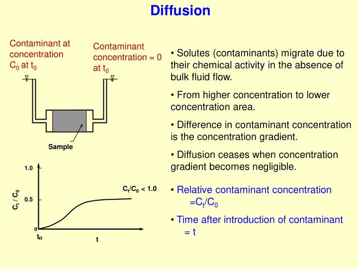
- Solutes (contaminants) migrate due to
their chemical activity in the absence of bulk fluid flow.
- From higher concentration to lower
concentration area.
- Difference in contaminant concentration
is the concentration gradient.
- Diffusion ceases when concentration
gradient becomes negligible.
Contaminant at concentration C0 at t0 Contaminant concentration = 0 at t0
Sample
- Time after introduction of contaminant
= t
- Relative contaminant concentration
=Ct/C0
Diffusion
1.0 0.5
t
Ct/C0 < 1.0 Ct / C0
SLIDE 2 Diffusion
- Add small amount of dye in a fluid
- Pulse gets spread out
Add continuous dye-- a sharp front
SLIDE 3 Types of Diffusion
- Steady State Diffusion
- Diffusion flux constant with time
- Fick’s First law applicable
- Non Steady-state Diffusion
- Concentration gradient non-uniform
- Follows Fick’s second law
x t x C D x t t x C , ,
JD =-D..(C/x)
D = diffusion coefficient [L2/T] = porosity C/x = concentration gradient (i.e., change in concentration with distance)
SLIDE 4 Chemical Energy Field
- To study the mechanism(s) of contaminant transport –
- the intact and fractured rock samples (Gurumoorthy 2002)
- diffusion characteristics of the saturated and unsaturated
soils (Rakesh 2005)
- Investigations using the Cl-, I+2, Cs+1 and Sr+2 in their active
as well as inactive forms
- Development of Diffusion Cell
SLIDE 5 CONTAMINANT TRANSPORT MODELING THROUGH THE ROCK MASS
Fractured Rock mass (FRM) Co Ct Intact Rock mass (IRM) C0 Ct Ct
Diffusion cells
SLIDE 6 7 min. 50 days 6 m thick FRM 75 min. 520 days 0.3 m thick IRM (Di)m=(Di)p
α
α
2000 4000 6000 8000 10000 10 20 30 40 Intact rock mass 2000 4000 6000 8000 10000
C
t
/C
0 (x10
Fractured rock mass
N 33 50 75 100
Time (s)
1 10 100 10
1
10
2
10
3
10
4
10
5
10
6
y=1.8
Intact rock mass Fractured rock mass
y=1.97
Diffusion time (s)
N
tm=tp.N-2
Diffusion characteristics
Fractured Rock mass (FRM) Co Ct Intact Rock mass (IRM) C0 Ct Ct
Diffusion cells
CONTAMINANT TRANSPORT MODELING THROUGH THE ROCK MASS
SLIDE 7 70
30
U C 60 A A B B
60
Modeling Diffusion in soils using impedance spectroscopy (IS)
Diffusion cell Impedance value of the soil is measured by using LCR meter Diffusion of contaminant can be monitored by determining the change in the impedance of the soil
SLIDE 8
100 200 300 400 500 10 20 30 40
(a)
453
Ct/C0 (x10
t (h)
- The slope of the break-through curve diffusion coefficient, D
- Archie’s law (D=.m) porosity of the geomaterials
SLIDE 9 Details of the diffusion studies Overall four cells were employed for each sample Z' measurement corresponding to 3rd, 6th, 9th and 20th day 1 M NaCl and 0.01 M SrCl2 used as model contaminants Na+ and Sr+2 analysis using AAS along the length of the cell
Soil Sample d (kN/m3) Sr (%) w (%) Θ (%) WC WC 100 13.8 100 80 60 33 45.54 WC 80 14.0 27 37.8 WC 60 13.8 22 30.36 CS CS 100 14.7 29 42.63 CS 80 14.9 23 34.27 CS 60 14.4 18 25.92
SLIDE 10 With time Ct increases on U due to diffusion Implies Z ′ decreases on U with time
Z′
t
C 1
Ct Contamination
1 2 3 4 5 6 7 8 9 10 11 500 1000 1500 2000 2500 3000 3500 4000 4500 5000 C WC 60-N
Time (Days) 3 6 9
Z' ( W ) Length (cm) U
General observations
Influence of Saturation
For a time t, Diffusion decreases with decreasing saturation
1 2 3 4 5 6 7 8 9 10 11 500 1000 1500 2000 2500 3000 3500 4000 4500 5000
C
9
th
day WC 60-N WC 80-N WC 100-N
Z' ( W ) Length (cm) U
SLIDE 11 (Normalized concentration) Ct/C0 vs Length
c c 1 m 2 c d 2 2 e c t
L mx sin L mx cos . m ) L R / t m D exp( 2 L x C C
(Diffusion coefficient) De vs volumetric water content