SLIDE 7 7 Modifying Perceptron Learning
} T
- minimize error, we can modify the algorithm slightly:
1.
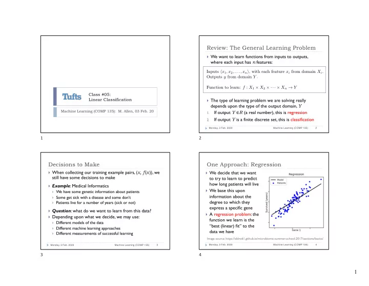
Choose an input xi from our data set that is wrongly classified.
2.
Update vector of weights, , as follows:
3.
Repeat until no classification errors remain.
3.
Repeat until weights no longer change; modify learning parameter 𝛽 over time to guarantee this.
} If we make 𝛽 smaller and smaller over time, then as ,
the weights will quit changing, and the algorithm converges
} T
- get down to a least-error possible final separator, we do this
slowly, e.g., setting , where t is the current iteration of the update algorithm
Monday, 3 Feb. 2020 Machine Learning (COMP 135) 25
w = (w0, w1, w2, . . . , wn)
wj ← wj + α(yi − hw(xi)) × xi,j α → 0 α(t) = 1000/(1000 + t) 25
Modifying Perceptron Learning
Monday, 3 Feb. 2020 Machine Learning (COMP 135) 26 Image source: Russel & Norvig, AI: A Modern Approach (Prentice Hal, 2010)
26
The History of the Perceptron
Monday, 3 Feb. 2020 Machine Learning (COMP 135) 27
Figure 4.8 Illustration of the Mark 1 perceptron hardware. The photograph on the left shows how the inputs were obtained using a simple camera system in which an input scene, in this case a printed character, was illuminated by powerful lights, and an image focussed onto a 20 × 20 array of cadmium sulphide photocells, giving a primitive 400 pixel image. The perceptron also had a patch board, shown in the middle photograph, which allowed different configurations of input features to be tried. Often these were wired up at random to demonstrate the ability of the perceptron to learn without the need for precise wiring, in contrast to a modern digital computer. The photograph on the right shows one of the racks of adaptive weights. Each weight was implemented using a rotary variable resistor, also called a potentiometer, driven by an electric motor thereby allowing the value of the weight to be adjusted automatically by the learning algorithm.
Frank Rosenblatt
1928–1969 Rosenblatt’s perceptron played an important role in the history of ma- chine learning. Initially, Rosenblatt simulated the perceptron on an IBM 704 computer at Cornell in 1957, but by the early 1960s he had built special-purpose hardware that provided a direct, par- allel implementation of perceptron learning. Many of his ideas were encapsulated in “Principles of Neuro- dynamics: Perceptrons and the Theory of Brain Mech- anisms” published in 1962. Rosenblatt’s work was criticized by Marvin Minksy, whose objections were published in the book “Perceptrons”, co-authored with Seymour Papert. This book was widely misinter- preted at the time as showing that neural networks were fatally flawed and could only learn solutions for linearly separable problems. In fact, it only proved such limitations in the case of single-layer networks such as the perceptron and merely conjectured (in- correctly) that they applied to more general network
- models. Unfortunately, however, this book contributed
to the substantial decline in research funding for neu- ral computing, a situation that was not reversed un- til the mid-1980s. Today, there are many hundreds, if not thousands, of applications of neural networks in widespread use, with examples in areas such as handwriting recognition and information retrieval be- ing used routinely by millions of people.
From: C. Bishop, Pattern Recognition and Machine
- Learning. Springer (2006).
27
This Week
} Linear classification; evaluating algorithms } Readings:
} Book excerpts on linear methods and evaluation metrics
} Posted to Piazza, linked from class schedule
} Assignment 02: due Wednesday, 12 Feb. } Office Hours: 237 Halligan
} Monday, Noon – 1:30 PM } Tuesday, 9:00 AM – 10:30 AM
Monday, 3 Feb. 2020 Machine Learning (COMP 135) 28
28