Today Making Simple Decisions Making Decisions Making Sequential - PDF document

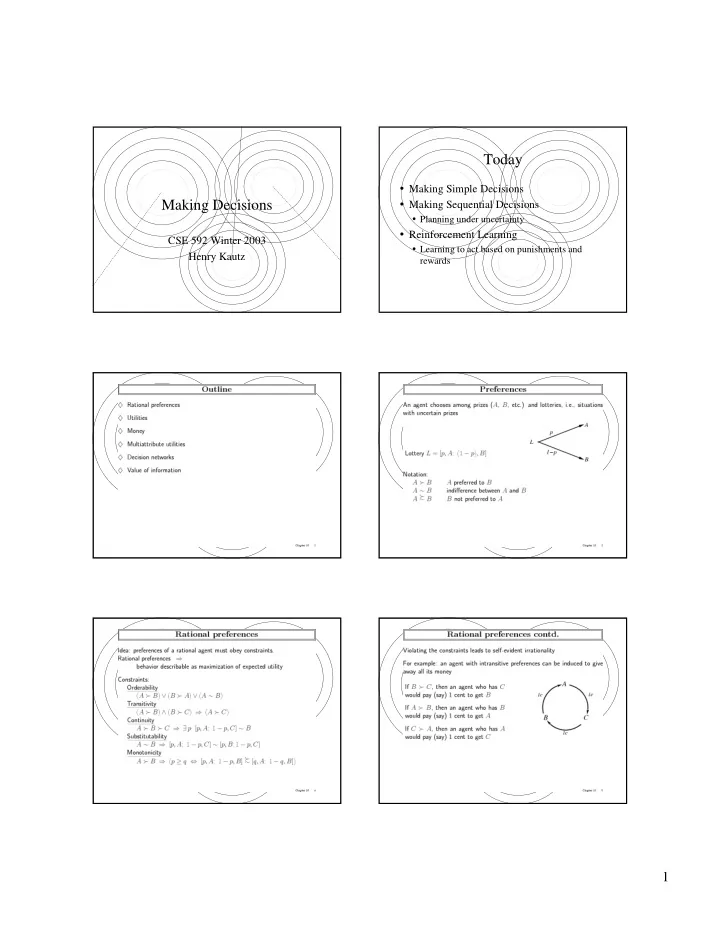
Today • Making Simple Decisions Making Decisions • Making Sequential Decisions • Planning under uncertainty • Reinforcement Learning CSE 592 Winter 2003 • Learning to act based on punishments and Henry Kautz rewards 1

2

Summary • Rational preferences yields utility theory • MEU: maximize expected utility • Highest expected reward over time • Not only possible decision rule! • Can map non-linear quantities (e.g. money) to linear utilities • Influence diagrams = Bayes net + decision nodes: MEU • Can compute value of gaining information • Preferential independence yields utility functions that are linear combinations of state attributes Break 3

4

Error Bounds What’s Hard About MDP’s? • Error between true/estimated value of a state reduced by discount factor λ at each • MDP’s are only hard to solve if the state iteration space is large • Exponentially fast convergence • Suppose a state is described by a set of • But still takes a long time if λ close to 1 propositional variables ( e.g., probabilistic • Optimal policy often found long before version of STRIPS planning) • Current research topic: performing value or state utility estimates converge policy iteration directly on a (small) representation of a large state space • Dan Weld & Mausam 2003 Multi-Agent MDP’s What’s Hard About MDP’s? • Payoff matrix – specify rewards 2 or more agents receive after each performs an action • MDP’s are only hard to solve if the state space is large Alice: testify Alice: refuse • Suppose world is only partially observed Bob: testify A=-5, B=-5 A=-10, B=0 • Agent assigns a probability distribution over Bob: refuse A=0, B=-10 A=-1, B=-1 possible values to each variable • “State” for the MDP becomes the agent’s state • Game theory – von Neuman – every zero- of belief – exponentially larger! sum game has an optimal mixed (stochastic) • No truly practical algorithms for general POMDP’s (yet) strategy 5

Summary • Markov Decision Processes provide a general way of reasoning about sequential decision problems • Solved by linear programming, value iteration, or policy iteration Break • Discounting future rewards guarantees convergence of value/policy iteration • Requires complete model of the world ( i.e. the state transition function) • MPD – complete observations • POMDP – partial observations • Large state spaces problematic Reinforcement Learning The Reinforcement Learning • “Of several responses made to the same situation, those Scenario which are accompanied or closely followed by satisfaction to the animal will, other things being equal, be more firmly • How is learning to act possible when… connected with the situation, so that, when it recurs, they will be more likely to recur; those which are accompanied or • Actions have non-deterministic effects, that are closely followed by discomfort to the animal will, other initially unknown things being equal, have their connections with that situation weakened, so that, when it recurs, they will be less likely to • Rewards or punishments come infrequently, at occur. The greater the satisfaction or discomfort, the greater the end of long sequences of actions the strengthening or weakening of the bond.” (Thorndike, • The learner must decide what actions to take 1911, p. 244) • The world is large and complex RL Techniques Passive RL • Temporal-difference learning • Given policy π , estimate U π (s) • Learns a utility function on states or on [state,action] • Not given transition matrix or pairs • Similar to backpropagation – treats the difference reward function! between expected / actual reward as an error signal, that is propagated backward in time • Epochs: training sequences • Exploration functions • Balance exploration / exploitation (1,1) ! (1,2) ! (1,3) ! (1,2) ! (1,3) ! (1,2) ! (1,1) ! (1,2) ! (2,2) ! (3,2) –1 • Function approximation (1,1) ! (1,2) ! (1,3) ! (2,3) ! (2,2) ! (2,3) ! (3,3) +1 (1,1) ! (1,2) ! (1,1) ! (1,2) ! (1,1) ! (2,1) ! (2,2) ! (2,3) ! (3,3) +1 • Compress a large state space into a small one (1,1) ! (1,2) ! (2,2) ! (1,2) ! (1,3) ! (2,3) ! (1,3) ! (2,3) ! (3,3) +1 • Linear function approximation, neural nets, … (1,1) ! (2,1) ! (2,2) ! (2,1) ! (1,1) ! (1,2) ! (1,3) ! (2,3) ! (2,2) ! (3,2) -1 • Generalization (1,1) ! (2,1) ! (1,1) ! (1,2) ! (2,2) ! (3,2) -1 6

Approaches Approaches • Adaptive Dynamic Programming • Direct estimation • Requires fully observable environment • Estimate U π (s) as average total reward of • Estimate transition function M from training data epochs containing s (calculating from s to end • Apply modified policy iteration to solve of epoch) Bellman equation: • Requires huge amount of data – does not take + ∑ π π π = λ ′ U R s ( ) M U ( ) s advantage of Bellman constraints! ′ s s , ′ • Expected utility of a state = its own reward + s expected utility of its successor states • Drawbacks: requires complete observations, and you don’t usually need value of all states Temporal Difference Learning Example: • Ideas • Do backups on a per-epoch basis • Don’t even try to estimate entire transition function! • For each transition from s to s’, update: π π π π ← + α + λ ′ − U ( ) s U ( ) s ( ( ) R s U ( s ) U ( )) s Q-Learning Active Reinforcement Learning • Version of TD-learning where instead of learning a value function on states, we learn • Suppose agent has to create its own policy one on [state,action] pairs while learning • First approach: π π π ′ − π ← + α + λ U ( ) s U ( ) s ( ( ) R s U ( ) s U ( ) s ) • Start with arbitrary policy beco m e s • Apply Q-Learning ← + α + ′ ′ − Q a ( , ) s Q a s ( , ) ( ( ) R s max Q a s ( , ) Q ( , a s ) ) • New policy: in state s , choose action a that ′ a maximizes Q(a,s) • Problem? • Why do this? 7

Exploration Functions Function Approximation • Problem of large state spaces remain • Too easily stuck in non-optimal space • Never enough training data! • Simple fix: with fixed probability perform a • Want to generalize what has been learned to random action new situations • Better: increase estimated expected value of • Idea: states that have been rarely explored • Replace large state table by a smaller, • “Exploration versus exploitation tradeoff” parameterized function • Updating the value of state will change the value assigned to many other similar states Linear Function Approximation Neural Nets • Represent U(s) as a weighted sum of • Neural nets can be used to create powerful features (basis functions) of s function approximators • Can become unstable (unlike linear ˆ ( ) = θ + θ + + θ U s f s ( ) f ( ) s ... f ( ) s θ 1 1 2 2 n n functions) • For TD-learning, apply difference signal to • Update each parameter separately, e.g: neural net output and perform back- ˆ ( ) ∂ U s propagation ˆ ˆ ′ θ θ ← θ + α + λ − ( ( ) R s U ( ) s U ( ) s ) θ θ i i ∂ θ i Example Demo 8

Summary • Use reinforcement learning when model of world is unknown and/or rewards are delayed • Temporal difference learning is a simple and efficient training rule • Q-learning eliminates need to ever use an explicit model of the transition function • Large state spaces can (sometimes!) be handled by function approximation, using linear functions or neural nets 9