Dynamic Programming Sequence Of Decisions Sequence of decisions. - PDF document

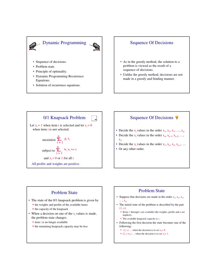
Dynamic Programming Sequence Of Decisions • Sequence of decisions. • As in the greedy method, the solution to a problem is viewed as the result of a • Problem state. sequence of decisions. • Principle of optimality. • Unlike the greedy method, decisions are not • Dynamic Programming Recurrence made in a greedy and binding manner. Equations. • Solution of recurrence equations. 0/1 Knapsack Problem Sequence Of Decisions Let x i = 1 when item i is selected and let x i = 0 when item i is not selected. • Decide the x i values in the order x 1 , x 2 , x 3 , …, x n . • Decide the x i values in the order x n , x n-1 , x n-2 , …, n p i x i x 1 . maximize i = 1 • Decide the x i values in the order x 1 , x n , x 2 , x n-1 , … n • Or any other order. w i x i <= c subject to i = 1 and x i = 0 or 1 for all i All profits and weights are positive. Problem State Problem State • Suppose that decisions are made in the order x 1 , x 2 , x 3 , • The state of the 0/1 knapsack problem is given by …, x n . • The initial state of the problem is described by the pair � the weights and profits of the available items (1, c). � the capacity of the knapsack � Items 1 through n are available (the weights, profits and n are • When a decision on one of the x i values is made, implicit). the problem state changes. � The available knapsack capacity is c. � item i is no longer available • Following the first decision the state becomes one of the following: � the remaining knapsack capacity may be less � (2, c) … when the decision is to set x 1 = 0. � (2, c-w 1 ) … when the decision is to set x 1 = 1.

Problem State Principle Of Optimality • Suppose that decisions are made in the order x n , x n-1 , x n-2 , • An optimal solution satisfies the following …, x 1 . property: • The initial state of the problem is described by the pair (n, c). � No matter what the first decision, the remaining � Items 1 through n are available (the weights, profits and first decisions are optimal with respect to the state that item index are implicit). results from this decision. � The available knapsack capacity is c. • Dynamic programming may be used only when • Following the first decision the state becomes one of the following: the principle of optimality holds. � (n-1, c) … when the decision is to set x n = 0. � (n-1, c-w n ) … when the decision is to set x n = 1. 0/1 Knapsack Problem x 1 = a 1 = 0 • Suppose that decisions are made in the order x 1 , n p i x i x 2 , x 3 , …, x n . maximize i = 2 • Let x 1 = a 1 , x 2 = a 2 , x 3 = a 3 , …, x n = a n be an n optimal solution. w i x i <= c subject to i = 2 • If a 1 = 0, then following the first decision the state is (2, c). and x i = 0 or 1 for all i • a 2 , a 3 , …, a n must be an optimal solution to the • If not, this instance has a better solution b 2 , b 3 , knapsack instance given by the state (2,c). …, b n . n n p i a i p i b i > i = 2 i = 2 x 1 = a 1 = 0 x 1 = a 1 = 1 • Next, consider the case a 1 = 1. Following the • x 1 = a 1 , x 2 = b 2 , x 3 = b 3 , …, x n = b n is a better first decision the state is (2, c-w 1 ). solution to the original instance than is x 1 = • a 2 , a 3 , …, a n must be an optimal solution to a 1 , x 2 = a 2 , x 3 = a 3 , …, x n = a n . the knapsack instance given by the state (2,c • So x 1 = a 1 , x 2 = a 2 , x 3 = a 3 , …, x n = a n cannot -w 1 ). be an optimal solution … a contradiction with the assumption that it is optimal.

x 1 = a 1 = 1 x 1 = a 1 = 1 n • x 1 = a 1 , x 2 = b 2 , x 3 = b 3 , …, x n = b n is a better p i x i maximize solution to the original instance than is x 1 = a 1 , x 2 = i = 2 a 2 , x 3 = a 3 , …, x n = a n . n • So x 1 = a 1 , x 2 = a 2 , x 3 = a 3 , …, x n = a n cannot be an w i x i <= c- w 1 subject to i = 2 optimal solution … a contradiction with the assumption that it is optimal. and x i = 0 or 1 for all i • If not, this instance has a better solution b 2 , b 3 , …, b n . n n p i a i p i b i > i = 2 i = 2 0/1 Knapsack Problem Dynamic Programming Recurrence • Therefore, no matter what the first decision, the • Let f(i,y) be the profit value of the optimal solution to remaining decisions are optimal with respect to the knapsack instance defined by the state (i,y). the state that results from this decision. � Items i through n are available. • The principle of optimality holds and dynamic � Available capacity is y. programming may be applied. • For the time being assume that we wish to determine only the value of the best solution. � Later we will worry about determining the x i s that yield this maximum value. • Under this assumption, our task is to determine f(1,c). Dynamic Programming Recurrence Dynamic Programming Recurrence • Suppose that i < n. • f(n,y) is the value of the optimal solution to the knapsack instance defined by the state (n,y). • f(i,y) is the value of the optimal solution to the knapsack instance defined by the state (i,y). � Only item n is available. � Items i through n are available. � Available capacity is y. � Available capacity is y. • If w n <= y, f(n,y) = p n . • Suppose that in the optimal solution for the state • If w n > y, f(n,y) = 0. (i,y), the first decision is to set x i = 0. • From the principle of optimality (we have shown that this principle holds for the knapsack problem), it follows that f(i,y) = f(i+1,y).

Recursive Code Dynamic Programming Recurrence /** @return f(i,y) */ • The only other possibility for the first decision private static int f(int i, int y) is x i = 1. { • The case x i = 1 can arise only when y >= w i . if (i == n) return (y < w[n]) ? 0 : p[n]; • From the principle of optimality, it follows that if (y < w[i]) return f(i + 1, y); f(i,y) = f(i+1,y-w i ) + p i . return Math.max(f(i + 1, y), • Combining the two cases, we get f(i + 1, y - w[i]) + p[i]); � f(i,y) = f(i+1,y) whenever y < w i . } � f(i,y) = max{f(i+1,y), f(i+1,y-w i ) + p i }, y >= w i . Recursion Tree Time Complexity • Let t(n) be the time required when n items are available. f(1,c) • t(0) = t(1) = a, where a is a constant. • When t > 1, f(2,c ) f(2,c-w 1 ) t(n) <= 2t(n-1) + b, f(3,c) f(3,c-w 2 ) f(3,c-w 1 ) f(3,c-w 1 –w 2 ) where b is a constant. • t(n) = O(2 n ). f(4,c) f(4,c-w 3 ) f(4,c-w 2 ) f(4,c-w 1 –w 3 ) Solving dynamic programming recurrences f(5,c) recursively can be hazardous to run time. f(5,c-w 1 –w 3 –w 4 ) Time Complexity Reducing Run Time • Level i of the recursion tree has up to 2 i-1 nodes. • At each such node an f(i,y) is computed. f(1,c) • Several nodes may compute the same f(i,y). • We can save time by not recomputing already f(2,c ) f(2,c-w 1 ) computed f(i,y)s. • Save computed f(i,y)s in a dictionary. f(3,c) f(3,c-w 2 ) f(3,c-w 1 ) f(3,c-w 1 –w 2 ) � Key is (i, y) value. � f(i, y) is computed recursively only when (i,y) is not in f(4,c) f(4,c-w 3 ) f(4,c-w 2 ) f(4,c-w 1 –w 3 ) the dictionary. f(5,c) � Otherwise, the dictionary value is used. f(5,c-w 1 –w 3 –w 4 )

Integer Weights Integer Weights Dictionary • Assume that each weight is an integer. • Use an array fArray[][] as the dictionary. • The knapsack capacity c may also be assumed • fArray[1:n][0:c] to be an integer. • fArray[i][y] = -1 iff f(i,y) not yet computed. • Only f(i,y)s with 1 <= i <= n and 0 <= y <= c • This initialization is done before the recursive method is invoked. are of interest. • The initialization takes O(cn) time. • Even though level i of the recursion tree has up to 2 i-1 nodes, at most c+1 represent different f(i,y)s. No Recomputation Code Time Complexity private static int f(int i, int y) • t(n) = O(cn). { • Analysis done in text. if (fArray[i][y] >= 0) return fArray[i][y]; • Good when cn is small relative to 2 n . if (i == n) {fArray[i][y] = (y < w[n]) ? 0 : p[n]; • n = 3, c = 1010101 return fArray[i][y];} w = [100102, 1000321, 6327] if (y < w[i]) fArray[i][y] = f(i + 1, y); p = [102, 505, 5] else fArray[i][y] = Math.max(f(i + 1, y), • 2 n = 8 f(i + 1, y - w[i]) + p[i]); • cn = 3030303 return fArray[i][y]; }