Dead Code Elimination & Dead code elimination Constant - - PowerPoint PPT Presentation

dead code elimination
SMART_READER_LITE
LIVE PREVIEW

Dead Code Elimination & Dead code elimination Constant - - PowerPoint PPT Presentation

Dead Code Elimination on SSA Form Dead Code Elimination & Dead code elimination Constant Propagation Conceptually similar to mark-sweep garbage collection C t ll i il t k b ll ti > Mark useful operations on SSA Form SSA F


slide-1
SLIDE 1

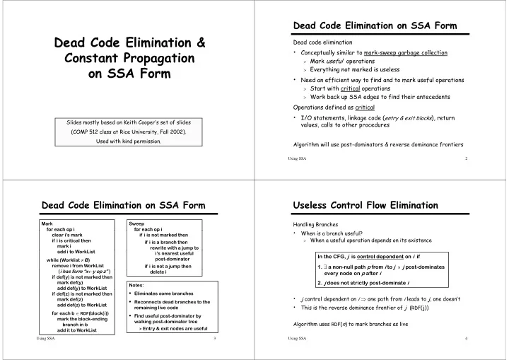
Dead Code Elimination & Constant Propagation SSA F

  • n SSA Form

Slides mostly based on Keith Cooper’s set of slides ( l ll ) (COMP 512 class at Rice University, Fall 2002). Used with kind permission.

Dead Code Elimination on SSA Form

Dead code elimination C t ll i il t k b ll ti

  • Conceptually similar to mark-sweep garbage collection

> Mark useful operations > Everything not marked is useless > Everything not marked is useless

  • Need an efficient way to find and to mark useful operations

> Start with critical operations > Start with critical operations > Work back up SSA edges to find their antecedents

Operations defined as critical p

  • I/O statements, linkage code (entry & exit blocks), return

values, calls to other procedures Algorithm will use post-dominators & reverse dominance frontiers

Using SSA 2

Dead Code Elimination on SSA Form

Mark for each op i Sweep for each op i for each op i clear i’s mark if i is critical then mark i dd i t W kLi t for each op i if i is not marked then if i is a branch then rewrite with a jump to add i to WorkList while (Worklist ≠ Ø) remove i from WorkList (i h f “ ” ) j p i’s nearest useful post-dominator if i is not a jump then (i has form “x←y op z” ) if def(y) is not marked then mark def(y) add def(y) to WorkList delete i Notes: add def(y) to WorkList if def(z) is not marked then mark def(z) add def(z) to WorkList

  • Eliminates some branches
  • Reconnects dead branches to the

remaining live code for each b ∈ RDF(block(i)) mark the block-ending branch in b dd it t W kLi t remaining live code

  • Find useful post-dominator by

walking post-dominator tree

> Entry & exit nodes are useful

Using SSA 3

add it to WorkList

> Entry & exit nodes are useful

Useless Control Flow Elimination

Handling Branches

  • When is a branch useful?

>

When a useful operation depends on its existence In the CFG, j is control dependent on i if

  • 1. ∃ a non-null path p from i to j ∋ j post-dominates

p p j j p every node on p after i

  • 2. j does not strictly post-dominate i
  • j control dependent on i ⇒ one path from i leads to j, one doesn’t
  • This is the reverse dominance frontier of j (RDF(j))

This is the reverse dominance frontier of j (RDF(j)) Algorithm uses RDF(n) to mark branches as live

Using SSA 4

slide-2
SLIDE 2

Dead Code Elimination on SSA Form

What’s left?

  • Algorithm eliminates useless definitions & some useless branches
  • Algorithm leaves behind empty blocks & extraneous control-flow

Algorithm from: Cytron, Ferrante, Rosen, Wegman, & Zadeck, Efficiently Computing St ti Si l A i t F d th Static Single Assignment Form and the Control Dependence Graph, ACM TOPLAS 13(4), October 1991 ith ti d t R b Shill

Two more issues

  • Simplifying control-flow

with a correction due to Rob Shillner

  • Eliminating unreachable blocks

Both are CFG transformations (no need for SSA)

Using SSA 5

*

Constant Propagation

Safety

  • Proves that name always has known value
  • Proves that name always has known value
  • Specializes code around that value

>

Moves some computations to compile time (⇒ code motion) m mp mp m ( )

>

Exposes some unreachable blocks (⇒ dead code) O t it Opportunity

  • Value ≠ ⊥ signifies an opportunity

Profitability

  • Compile-time evaluation is cheaper than run-time evaluation

p p

  • Branch removal may lead to block coalescing

(CLEAN)

>

If not, it still avoids the test & makes branch predictable

Using SSA 6

Sparse Constant Propagation on SSA Form

∀ expression, e V l ( ) {

TOP if its value is unknown

if it l i k Value(e) ← WorkList ← Ø ∀ SSA edge s = <u,v> if Value(u) ≠ TOP then

{

ci if its value is known

BOT if its value is known to vary

i e o is “a←b op v” or “a ←v op b” if Value(u) ≠ TOP then add s to WorkList while (WorkList ≠ Ø) remove s = <u v> from WorkList i.e., o is a←b op v or a ←v op b remove s = <u,v> from WorkList let o be the operation that uses v if Value(o) ≠ BOT then t ← result of evaluating o Evaluating a Φ-node: Φ(x1,x2,x3, … xn) is Value(x ) ∧Value(x ) Value(x ) t ← result of evaluating o if t ≠ Value(o) then ∀ SSA edge <o,x> add <o,x> to WorkList Value(x1) ∧Value(x2) Value(x3) ∧ ... ∧ Value(xn) Where TOP ∧ x = x ∀ x TOP ∧ x = x ∀ x ci ∧ cj = ci if ci = cj ci ∧ cj = BOT if ci ≠ cj

BOT ∧ x = BOT

∀ x Same result, fewer ∧ operations Performs ∧ only at Φ nodes

Using SSA 7 BOT ∧ x = BOT

∀ x Performs ∧ only at Φ nodes

Sparse Constant Propagation on SSA Form

How long does this algorithm take to halt?

  • Initialization is two passes

TOP

  • Initialization is two passes

>

|ops| + 2 x |ops| edges

  • Value(x) can take on 3 values

BOT ci cj ck cl cm cn ... ...

( )

>

TOP, ci, BOT

>

Each use can be on WorkList twice 2 x | r s| 4 x | ps| ev lu ti ns W rkList pushes & p ps

BOT >

2 x |args| = 4 x |ops| evaluations, WorkList pushes & pops This is an optimistic algorithm: This is an optimistic algorithm:

  • Initialize all values to TOP, unless they are known constants
  • Every value becomes BOT or ci unless its use is uninitialized

Every value becomes BOT or ci, unless its use is uninitialized

Using SSA 8

slide-3
SLIDE 3

Sparse Conditional Constant Propagation

Optimism Optimism

12

⊥ Pessimistic initializations i0 ← 12 while ( … ) i1 ← Φ(i0 i3) Clear that i is

p

  • This version of the algorithm is

an optimistic formulation

12

TOP

Optimistic initializations ⊥ ⊥ ⊥ ⊥ Leads to: i1 ≡ 12 ∧ ⊥ ≡ ⊥ x ≡ ⊥ * 17 ≡ ⊥ j i1 ← Φ(i0,i3) x ← i1 * 17 j ← i1 i2 ← … always 12 at def of x

  • Initializes values to TOP
  • Prior version used ⊥

(implicit)

TOP TOP TOP TOP

Leads to: i1 ≡ 12 ∧ TOP ≡ 12 x ≡ 12 * 17 ≡ 204 j 12 ⊥ j ≡ ⊥ i3 ≡ ⊥ … i3 ← j

In general (implicit)

TOP

j ≡ 12 i3 ≡ 12 i1 ≡ 12 ∧ 12 ≡ 12

  • Optimism helps inside loops
  • Largely a matter of initial value

M.N. Wegman & F.K. Zadeck, Constant propagation with conditional branches ACM TOPLAS 13(2) April 1991 pages 181 210 Using SSA 9 branches, ACM TOPLAS, 13(2), April 1991, pages 181–210.

*

Sparse Conditional Constant Propagation

What happens when it propagates a value into a branch?

P

i k l d

  • TOP ⇒ we gain no knowledge
  • BOT ⇒ either path can execute

}

But, the algorithm does not use this

  • TRUE or FALSE ⇒ only one path can execute} does not use this ...

Working this into the algorithm kl k & FG k

  • Use two worklists: SSAWorkList & CFGWorkList

> SSAWorkList determines values > CFGWorkList governs reachability > CFGWorkList governs reachability

  • Don’t propagate into operation until its block is reachable

Using SSA 10

Sparse Conditional Constant Propagation

SSAWorkList ← Ø C GW kLi while ((CFGWorkList ∪ SSAWorkList) ≠ Ø) CFGWorkList ← n0 ∀ block b clear b’s mark ∀ expression e in b while(CFGWorkList ≠ Ø) remove b from CFGWorkList mark b evaluate each Φ function in b ∀ expression e in b Value(e) ← TOP Initialization Step evaluate each Φ-function in b evaluate each op in b, in order while(SSAWorkList ≠ Ø) remove s = <u v> from WorkList p

To evaluate a branch if arg is BOT then

remove s = <u,v> from WorkList let o be the operation that contains v t ← result of evaluating o if t V l ( ) th

if arg is BOT then put both targets on CFGWorklist else if arg is TRUE then put TRUE target on CFGWorkList l if i FALSE th

if t ≠ Value(o) then Value(o) ← t ∀ SSA edge <o,x> if x is marked, then

else if arg is FALSE then put FALSE target on CFGWorkList To evaluate a jump place its target on CFGWorkList

if x is marked, then add <o,x> to WorkList Propagation Step

Using SSA 11 p g

Sparse Conditional Constant Propagation

There are some subtle points B h diti h ld t b TOP h l t d

  • Branch conditions should not be TOP when evaluated

> Indicates an upwards-exposed use

(no initial value)

> Hard to envision compiler producing such code > Hard to envision compiler producing such code

  • Initialize all operations to TOP

Bl k i ill fill i th t i iti l l

> Block processing will fill in the non-top initial values > Unreachable paths contribute TOP to Φ-functions

  • Code shows CFG edges first, then SSA edges

> Can intermix them in arbitrary order

(correctness)

T ki CFG d fi t h l ith d ( i

ff )

> Taking CFG edges first may help with speed (minor effect)

Using SSA 12

slide-4
SLIDE 4

Sparse Conditional Constant Propagation

More subtle points

  • TOP * BOT → TOP
  • TOP * BOT → TOP

>

If TOP becomes 0, then 0 * BOT → 0

>

This prevents non-monotonic behavior for the result value

>

Uses of the result value might go irretrievably to

>

Similar effects with any operation that has a “zero”

  • Some values reveal simplifications, rather than constants

>

BOT * ci → BOT, but might turn into shifts & adds (ci = 2, BOT ≥ 0)

>

Removes commutativity (reassociation)

>

Removes commutativity (reassociation)

>

BOT**2 → BOT * BOT

(vs. series or call to library)

  • cbr TRUE → L L

becomes br → L

  • cbr TRUE → L1,L2 becomes br → L1

>

Method discovers this; it must rewrite the code, too!

Using SSA 13

Sparse Conditional Constant Propagation

Unreachable Code Optimism p

  • Initialization to TOP is still

important

i ← 17 if (i > 0) then j1 ← 10 All paths execute

10 17

With SCC marking blocks

17

TOP

10

  • Unreachable code keeps TOP
  • ∧ with TOP has desired result

j1 ← 1 else j2 ← 20 j3 ← Φ(j1, j2)

20 ⊥

TOP TOP

10 10

Cannot get this any other way

  • DEAD code cannot test (i > 0)

k ← j3 * 17

⊥ 170

  • DEAD marks j2 as useful

In general, combining two optimizations can lead to answers that cannot be produced by any combination of running them separately. This algorithm is one example of that general principle. C bi i i ll i & i i h d li i h

Using SSA 14

*

Combining register allocation & instruction scheduling is another ...

Using SSA Form for Optimizations

In general, using SSA conversion prior to optimization leads to Cl f l ti

  • Cleaner formulations
  • Better results
  • Faster algorithms

We’ve seen two SSA-based optimization algorithms D d d l

  • Dead-code elimination
  • Sparse conditional constant propagation

There are many more…

Using SSA 15