[PDF] - Informed Search How can we make search smarter? Use PDF Document

SLIDE 1

1

CS 331: Artificial Intelligence Informed Search

2

Informed Search

How can we make search smarter?
Use problem-specific knowledge beyond

the definition of the problem itself

Specifically, incorporate knowledge of how

good a non-goal state is

3

Best-First Search

Node selected for expansion based on an

evaluation function f(n). i.e. expand the node that appears to be the best

Node with lowest evaluation is selected for

expansion

Uses a priority queue
We’ll talk about Greedy Best-First Search

and A* Search

4

Heuristic Function

h(n) = estimated cost of the cheapest path

from node n to a goal node

h(goal node) = 0
Contains additional knowledge of the

problem

5

Greedy Best-First Search

Expands the node that is closest to the goal
f(n) = h(n)

6

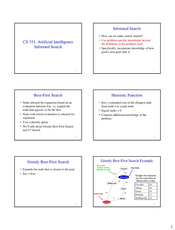
Greedy Best-First Search Example

Corvallis Albany Salem McMinnville Portland

Goal State Initial State

11 26 30 38 46 Wilsonville 18

Corvallis 56 Albany 49 Salem 28 Portland 17 McMinnville 18 Straight line distance (as the crow flies) to Wilsonville in miles

28

This is the “actual” driving distance in miles

SLIDE 2

2

7

Greedy Best-First Search Example

Corvallis 56

h(n)

Corvallis 56 Albany 49 Salem 28 Portland 17 McMinnville 18

8

Greedy Best-First Search Example

Corvallis McMinnville Albany 18 49

Corvallis 56 Albany 49 Salem 28 Portland 17 McMinnville 18

Greedy Best-First Search Example

Corvallis McMinnville Albany 49 Portland Wilsonville Corvallis 56 17

Corvallis →McMinnville→ Wilsonville = 74 miles Corvallis 56 Albany 49 Salem 28 Portland 17 McMinnville 18

Greedy Best-First Search Example

Corvallis →Albany→ Salem → Wilsonville = 67 miles

But the route below is much shorter than the route found by Greedy Best-First Search!

Corvallis Albany Salem McMinnville Portland

Goal State Initial State

11 26 30 38 46 Wilsonville 18 28

11

Evaluating Greedy Best-First Search

Complete? No (could start down an infinite path) Optimal? Time Complexity Space Complexity

12

Evaluating Greedy Best-First Search

Complete? No (could start down an infinite path) Optimal? No Time Complexity Space Complexity

Greedy Best-First search results in lots of dead ends which leads to unnecessary nodes being expanded

SLIDE 3

3

13

Evaluating Greedy Best-First Search

Complete? No (could start down an infinite path) Optimal? No Time Complexity O(bm) Space Complexity

Greedy Best-First search results in lots of dead ends which leads to unnecessary nodes being expanded

14

Evaluating Greedy Best-First Search

Complete? No (could start down an infinite path) Optimal? No Time Complexity O(bm) Space Complexity O(bm)

Greedy Best-First search results in lots of dead ends which leads to unnecessary nodes being expanded

15

A* Search

A much better alternative to greedy best-

first search

Evaluation function for A* is:

f(n) = g(n) + h(n) where g(n) = path cost from the start node to n

If h(n) satisfies certain conditions, A*

search is optimal and complete!

16

Admissible Heuristics

A* is optimal if h(n) is an admissible

heuristic

An admissible heuristic is one that never
verestimates the cost to reach the goal
Admissible heuristic = optimistic
Straight line distance was an admissible

heuristic

17

Greedy Best-First Search Example

Corvallis Albany Salem McMinnville Portland

Goal State Initial State

11 26 30 38 46 Wilsonville 18

Corvallis 56 Albany 49 Salem 28 Portland 17 McMinnville 18 Straight line distance (as the crow flies) to Wilsonville in miles

28

This is the “actual” driving distance in miles

18

A* Search Example

Corvallis 56=0+56

f(n)=g(n)+h(n)

Corvallis 56 Albany 49 Salem 28 Portland 17 McMinnville 18 Straight line distance (as the crow flies) to Wilsonville in miles

SLIDE 4

4

19

A* Search Example

Corvallis McMinnville Albany 46+18=64 11+49=60

Corvallis 56 Albany 49 Salem 28 Portland 17 McMinnville 18 Straight line distance (as the crow flies) to Wilsonville in miles

46 11

20

A* Search Example

Corvallis McMinnville Albany 46+18=64 Salem Corvallis 37+28=65 22+56=78

Corvallis 56 Albany 49 Salem 28 Portland 17 McMinnville 18

46 11 11 26

21

A* Search Example

Corvallis McMinnville Albany Salem Corvallis 37+28=65 22+56=78 Portland Wilsonville Corvallis 84+17=101 92+56=148 74+0=74

Note: Don’t stop when you put a goal state on the priority queue (otherwise you get a suboptimal solution)

46 11 11 26 38 46 28

A* Search Example

Corvallis McMinnville Albany Salem Corvallis 22+56=78 Portland Wilsonville Corvallis 84+17=101 92+56=148 74+0=74 Wilsonville Albany 67+0=67 63+49=112

Proper termination: Stop when you pop a goal state from the priority queue

46 38 46 11 11 26 28 30 26

23

Proof that A* using TREE-SEARCH is optimal if h(n) is admissible

Suppose A* returns a suboptimal goal node G2 .
G2 must be the least cost node in the fringe. Let

the cost of optimal solution be C*

Because G2 is suboptimal:

f(G2) = g(G2) + h(G2) = g(G2) > C*

Now consider a fringe node n on an optimal

solution path to the goal G

If h(n) is admissible then:

f(n) = g(n) + h(n) ≤ C*

We have shown that f(n) ≤ C* < f(G2), so G2 will

not get expanded before n. Henc A* must return an optimal solution.

h(G2) = 0 because it is a goal node

n G2 G C*

24

What about search graphs (more than one path to a node)?

What if we expand a state we’ve already seen?
Suppose we use the GRAPH-SEARCH solution

and not expand repeated nodes

Could discard the optimal path if it’s not the first
ne generated
One simple solution: ensure optimal path to any

repeated state is always the first one followed (like in Uniform-cost search)

Requires an extra requirement on h(n) called

consistency (or monotonicity)

SLIDE 5

5 Consistency

A heuristic is consistent if, for every node n and every

successor n’ of n generated by any action a: h(n) ≤ c(n,a,n’) + h(n’)

A form of the triangle inequality – each side of the triangle

cannot be longer than the sum of the two sides

Step cost of going from n to n’ by doing action a n n’ G c(n,a,n’) h(n’) h(n) n n’ G c(n,a,n’)=2 h(n’)=1 h(n)=2 n n’ G c(n,a,n’)=2 h(n’)=1 h(n)=4

CONSISTENT INCONSISTENT

26

Consistency

Every consistent heuristic is also admissible
A* using GRAPH-SEARCH is optimal if

h(n) is consistent

Most admissible heuristics are also

consistent

27

Consistency

Claim: If h(n) is consistent, then the values of f(n) along

any path are nondecreasing

Proof:

Suppose n’ is a successor of n. Want to show f(n’) ≥ f(n) Then g(n’) = g(n) + c(n,a,n’) for some a f(n’) = g(n’) + h(n’) = g(n) + c(n,a,n’) + h(n’) ≥ g(n) + h(n) = f(n)

Thus, the sequence of nodes expanded by A* is in

nondecreasing order of f(n)

First goal selected for expansion must be an optimal

solution since all later nodes will be at least as expensive

From defn of consistency: c(n,a,n’) + h(n’) ≥ h(n)

28

A* is Optimally Efficient

Among optimal algorithms that expand search

paths from the root, A* is optimally efficient for any given heuristic function

Optimally efficient: no other optimal algorithm is

guaranteed to expand fewer nodes than A*

– Fine print: except A* might possibly expand more nodes with f(n) = C* where C* is the cost of the optimal path – tie-breaking issues

Any algorithm that does not expand all nodes with

f(n) < C* runs the risk of missing the optimal solution

29

Evaluating A* Search

With a consistent heuristic, A* is complete, optimal and

ptimally efficient. Could this be the answer to our

searching problems?

30

Evaluating A* Search

With a consistent heuristic, A* is complete, optimal and

ptimally efficient. Could this be the answer to our

searching problems? The Dark Side of A*…

Time complexity is exponential (although it can be reduced significantly with a good heuristic) The really bad news: space complexity is exponential (usually need to store all generated states). Typically runs out of space on large-scale problems.

SLIDE 6

6 Summary of A* Search

Complete? Yes if h(n) is consistent, b is finite, and all step costs exceed some finite  1 Optimal? Time Complexity Space Complexity

1 Since f(n) is nondecreasing, we must eventually hit an f(n) = cost of the path to a

goal state

Summary of A* Search

Complete? Yes if h(n) is consistent, b is finite, and all step costs exceed some finite  1 Optimal? Yes if h(n) is consistent and admissible Time Complexity Space Complexity

1 Since f(n) is nondecreasing, we must eventually hit an f(n) = cost of the path to a

goal state

Summary of A* Search

Complete? Yes if h(n) is consistent, b is finite, and all step costs exceed some finite  1 Optimal? Yes if h(n) is consistent and admissible Time Complexity O(bd) (In the worst case but a good heuristic can reduce this significantly) Space Complexity

1 Since f(n) is nondecreasing, we must eventually hit an f(n) = cost of the path to a

goal state

Summary of A* Search

Complete? Yes if h(n) is consistent, b is finite, and all step costs exceed some finite  1 Optimal? Yes if h(n) is consistent and admissible Time Complexity O(bd) (In the worst case but a good heuristic can reduce this significantly) Space Complexity O(bd) – Needs O(number of states), will run out of memory for large search spaces

1 Since f(n) is nondecreasing, we must eventually hit an f(n) = cost of the path to a

goal state

35

Iterative Deepening A*

Use iterative deepening trick to reduce memory

requirements for A*

In each iteration do a “cost-limited” depth first

search.

– Cutoff is based on the f-cost (g+h) rather than the depth

After each iteration, the new cutoff is the

smallest f-cost that exceeded the cutoff in the previous iteration

Complete, Optimal but more costly than A* and can take a while to run with real- valued costs

36

Examples of heuristic functions

7 2 4 5 6 8 3 1 1 2 3 4 5 6 7 8 The 8-puzzle

Start State End State

Heuristic #1: h1 = number of misplaced tiles eg. start state has 8 misplaced tiles. This is an admissible heuristic

SLIDE 7

7

37

Examples of heuristic functions

7 2 4 5 6 8 3 1 1 2 3 4 5 6 7 8 The 8-puzzle

Start State End State

Heuristic #2: h2 = total Manhattan distance (sum of horizontal and vertical moves, no diagonal moves). Start state is 3+1+2+2+3+2+2+3=18 moves away from the end state. This is also an admissible heuristic.

38

Which heuristic is better?

h2 dominates h1. That is, for any node n, h2(n) ≥ h1(n).
h2 never expands more nodes than A* using h1 (except

possibly for some nodes with f(n) = C*)

Better to use h2 provided it doesn’t overestimate (i.e., it is also

admissible) and its computation time isn’t too expensive.

Proof: Let h1 and h2 be admissible heuristics. Every node with f(n) < C* will surely be expanded, since A* is optimal with an admissible heuristic. Since f(n) = g(n) + h(n), every node with h(n) < C*- g(n) will surely be expanded for either heuristic. Since h2 is at least as big as h1 for all nodes, every node expanded with A* using h2 will also be expanded with A* using h1. But h1 might expand other nodes as

well. In other words, we have h1(n) ≤ h2(n) < C*- g(n)

Which heuristic is better?

# nodes expanded Depth IDS A*(h1) A*(h2) 2 10 6 6 4 112 13 12 6 680 20 18 8 6384 39 25 10 47127 93 39 12 3644035 227 73 14 539 113 16 1301 211 18 3056 363 20 7276 676 22 18094 1219 24 39135 1641

From Russell and Norvig Figure 4.8 (Results averaged over 100 instances of the 8-puzzle for depths 2-24).

40

Inventing Admissible Heuristics

Relaxed problem: a problem with fewer

restrictions on the actions

The cost of an optimal solution to a relaxed

problem is an admissible heuristic for the original problem

If we relax the rules so that a square can move

anywhere, we get heuristic h1

If we relax the rules to allow a square to move to

any adjacent square, we get heuristic h2

41

What you should know

Be able to run A* by hand on a simple

example

Why it is important for a heuristic to be

admissible and consistent

Pros and cons of A*
How do you come up with heuristics
What it means for a heuristic function to