Curve Sketching Since we have graphing calculators, we can find the - - PDF document

Mt020.02 Slide 1 3/24/2000

raj

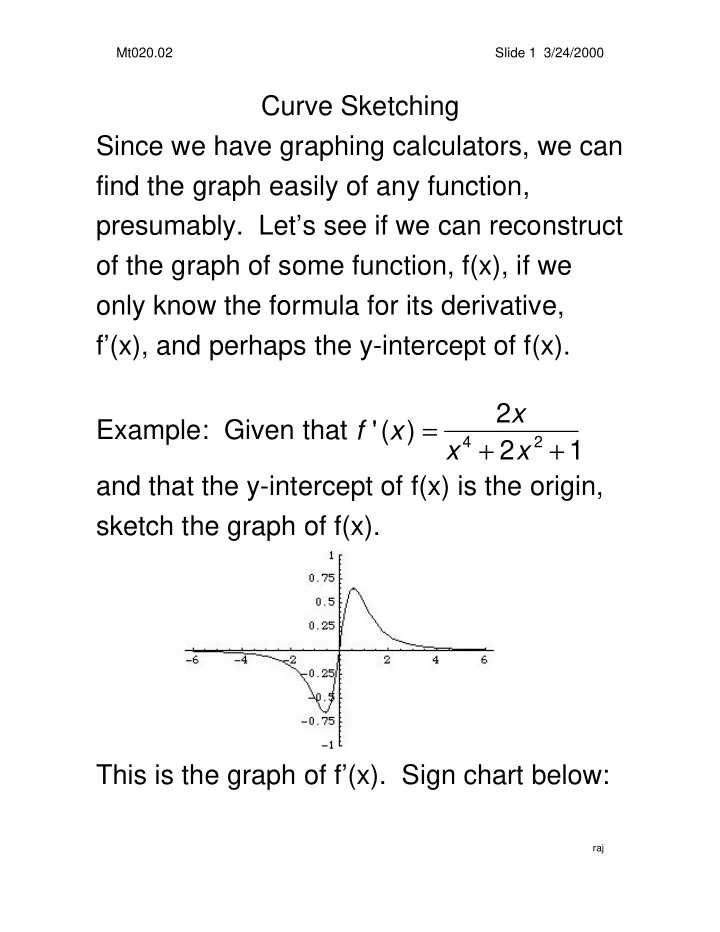
Curve Sketching Since we have graphing calculators, we can find the graph easily of any function,

• presumably. Let’s see if we can reconstruct
• f the graph of some function, f(x), if we
• nly know the formula for its derivative,

f’(x), and perhaps the y-intercept of f(x). Example: Given that f '(x) = 2x x 4 + 2x 2 + 1 and that the y-intercept of f(x) is the origin, sketch the graph of f(x). This is the graph of f’(x). Sign chart below:

Mt020.02 Slide 2 3/24/2000

raj

The function f itself will be decreasing until we hit zero and increasing thereafter. Because the derivative changes signs across zero, from – to +, we know that the point (0,f(0)) will turn out to be a relative minimum of f. This is the y-intercept, (0,0). ________________ We differentiate the function f’(x) to find the second derivative f’’(x) which holds the key to the concavity behavior of f(x). f '' (x) = 2 − 6x 2 ( 1 + x 2)3 . The graph of f’’ is Sign chart for f’’ below:

Mt020.02 Slide 3 3/24/2000

raj

Here is the assembly of our results: f is dec. for x<0 | f is inc. for x>0 x=0 f is ccd | f is ccu | f is ccd

• 0.577 0.577

Here’s our sketch:

Mt020.02 Slide 4 3/24/2000

raj

And the answer is f(x) = x 2 1+ x 2 and its graph ____________________________ Asymptotes are lines to which the graph

• f a function seems to adhere to as we

get further from the origin. In the previous example, our function had a horizontal asymptote y=1, because as we stray further from the origin the graph seems to be attracted by the line y=1. It is also possible to have vertical asymptotes at places where the function seems to want to be infinite. Like this:

Mt020.02 Slide 5 3/24/2000

raj

f(x) = 1 x − 2 This function has a vertical asymptote at x=2 and a horizontal asymptote y=0. Example: Find asymptotes for the function h(x) = 4x 2 − 2 x 2 −1 . We see that the denominator will be zero for x = ±1 and since those values do not make the numerator zero, we expect vertical asymptotes at x = ±1. And since

Mt020.02 Slide 6 3/24/2000

raj

lim x → ∞h(x) = lim x → ∞ 4x 2 − 2 x 2 − 1 = 4 we see that our graph should have horizontal asymptotes at y=4. Here’s a preliminary sketch of the playing field. If we differentiate h(x) we find that h' (x) = −4x (x 2 −1 )2 which has this shape:

Mt020.02 Slide 7 3/24/2000

raj

And this sign chart: h’(x) | | |

• 1 0 1

Note that h (and h’) are not defined at x=±1, which should both appear as critical points where the sign of the derivative could shift. We see h is max at x=0 and that h(0) = 2. Differentiating again we get formula and graphs for h’’: h' ' ( x) = 4(3x 2 +1 ) (x 2 −1 )3

Mt020.02 Slide 8 3/24/2000

raj

Sign chart for h’’ h’’ | |

• 1

1 Here’s our sketch putting all of our information together:

Mt020.02 Slide 9 3/24/2000

raj

And here is the real graph of h(x)