Main Effects vs. Simple Effects Scott Fraundorf MLM Reading Group - - PowerPoint PPT Presentation

Main Effects vs. Simple Effects

Scott Fraundorf MLM Reading Group April 7th, 2011

1 2 3 4 5 6 7 8 9 10 1 2 3 4 5 6 7 8 9 10

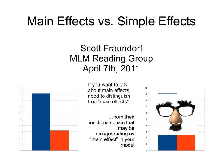
If you want to talk about main effects, need to distinguish true “main effects”... ...from their insidious cousin that may be masquerading as “main effect” in your model

Outline

 The Problem  Recap of Coding  Parameter Testing  Simple Effects & Main Effects  More Detailed Explanation  How to Do Contrast Coding  Continuous Predictors

Contrast Unmentioned

0.1 0.2 0.3 0.4 0.5 0.6 0.7 0.8 0.9 1

Presentational Contrastive

Prototypical psychology study: 2 x 2 design

Example Study

 Study easy and difficult word pairs

– VIKING—HELMET (related and thus easy) – VIKING—COLLEGE (unrelated and thus hard)

 Do cued recall task:

– VIKING---?????

 During test phase, told if an opponent

supposedly got the item correct or incorrect

Easy Items Hard Items

0.1 0.2 0.3 0.4 0.5 0.6 0.7 0.8 0.9 1

Opponent Correct Opponent Incorrect

Accuracy

INTERACTION!

Easy items are remembered better if the opponent supposedly got them right. Hard items are remembered better if the opponent got them wrong. (i.e., performance best in the MISMATCH conditions) Effect of feedback depends on item type (INTERACTION).

Easy Items Hard Items

0.1 0.2 0.3 0.4 0.5 0.6 0.7 0.8 0.9 1

Opponent Correct Opponent Incorrect

Accuracy

INTERACTION!

MAIN EFFECT Overall, the related (easy) items are also remembered better than the unrelated (hard) items

Easy Items Hard Items

0.1 0.2 0.3 0.4 0.5 0.6 0.7 0.8 0.9 1

Opponent Correct Opponent Incorrect

Accuracy

INTERACTION!

MAIN EFFECT MAIN EFFECT (OR LACK THEREOF) No consistent effect of

• pponent feedback.

The Problem

MLM WORLD ANOVA WORLD

• Get test of interaction
• And of 2 main effects
• Not in Kansas anymore!
• What to do?

The Problem

 Modeling our outcome variable in a regression

equation

 Need to code categorical

variables into numerical ones

 Consequences for how you

interpret hypothesis tests

β2X2 + β12X1X2 + ... Y=β0 β0+ β1X1 +

R's secret decoder wheel

Outline

 The Problem  Recap of Coding  Parameter Testing  Simple Effects & Main Effects  More Detailed Explanation  How to Do Contrast Coding  Continuous Predictors

OPPONENT FEEDBACK

Correct : 0 Incorrect : 1

DUMMY CODING a/k/a TREATMENT CODING (R's default)

ITEM TYPE

Related : 0 Unrelated : 1

One level is 1 Other level is 0

OPPONENT (A)

Didn't See : 0 Correct : 1 Incorrect : 0

OPPONENT (B)

Didn't See : 0 Correct : 0 Incorrect : 1

DUMMY CODING a/k/a TREATMENT CODING (R's default)

Predictor with >2 levels: get more dummy-coded variables ITEM TYPE

Related : 0 Unrelated : 1

DUMMY CODING CONTRAST CODING

ITEM TYPE

Related : -0.5 Unrelated : 0.5

OPPONENT FEEDBACK

Correct : -0.5 Incorrect : 0.5

One level is positive Other level is negative

One level is 1 Other level is 0 OPPONENT FEEDBACK

Correct : 0 Incorrect : 1

ITEM TYPE

Related : 0 Unrelated : 1

Outline

 The Problem  Recap of Coding  Parameter Testing  Simple Effects & Main Effects  More Detailed Explanation  How to Do Contrast Coding  Continuous Predictors

Testing a Parameter

β2X2 + ... Y=β0 β0+ β1X1 +

Feedback 0 = Correct 1 = Incorrect Item Type 0 = Related 1 = Unrelated

How to tell if the opponent's feedback is related to memory? (e.g. possible main effect: you just try harder when someone else got the item wrong)

Testing a Parameter

β2X2 + ... Y=β0 β0+ β10 +

Feedback 0 = Correct 1 = Incorrect Item Type 0 = Related 1 = Unrelated

Compare when feedback = 0...

Testing a Parameter

β2X2 + ... Y=β0 β0+ β11 +

Feedback 0 = Correct 1 = Incorrect Item Type 0 = Related 1 = Unrelated

… to when feedback = 1

Testing a Parameter

β2X2 + ... Y=β0 β0+ β1X1 +

Feedback 0 = Correct 1 = Incorrect Item Type 0 = Related 1 = Unrelated

β1: “The effect of changing feedback, while holding item type constant” But, we know there's an interaction … so it will matter what value we hold item type constant at!

Testing a Parameter

β2X2 + ... Y=β0 β0+ β1X1 +

Probe

With dummy coding, item type = 0 represents the RELATED condition. Testing effect of feedback in just the RELATED condition.

Feedback 0 = Correct 1 = Incorrect

Hold other variable at:

Easy Items Hard Items

0.1 0.2 0.3 0.4 0.5 0.6 0.7 0.8 0.9 1

Opponent Correct Opponent Incorrect

Accuracy

INTERACTION!

With dummy coding, item type = 0 represents the RELATED condition. Testing effect of feedback in just the RELATED condition. Hold other variable at: But, this test only reflects HALF of the graph! Here, we see Opponent Incorrect > Opponent Correct

Easy Items Hard Items

0.1 0.2 0.3 0.4 0.5 0.6 0.7 0.8 0.9 1

Opponent Correct Opponent Incorrect

Accuracy

INTERACTION!

Feedback effect is different in the other half. Misleading! But, this test only reflects HALF of the graph!

Outline

 The Problem  Recap of Coding  Parameter Testing  Simple Effects & Main Effects  More Detailed Explanation  How to Do Contrast Coding  Continuous Predictors

FEEDBACK

Correct : 0 Incorrect : 1

ITEM TYPE

Related : 0 Unrelated : 1

DUMMY CODING

What is effect of the Feedback variable? R holds Item Type at 0. Only reflects Related condition. Problem: Effect of Feedback depends on the Item Type. (i.e., there's an INTERACTION)

Simple Effect

FEEDBACK

Correct : -0.5 Incorrect : 0.5

ITEM TYPE

Related : -0.5 Unrelated : 0.5 CONTRAST CODING

What is effect of the Feedback variable? R holds Item Type at 0. Averaged between 2 conditions. Test now uses information from both Item Types in testing

• Feedback. (No main

effect here.)

Main Effect

 Dummy Coding -> Simple Effects

 Consider only one level of predictor X2 in testing

predictor X1

 Contrast Coding -> Main Effects

 Consider all levels of predictor X2 in testing

predictor X1

 Both are legitimate statistical tests, but they

test different things

– Simple effects may be appropriate if you WANT to only test at one level of predictor X2 – e.g. that level is the baseline (“opponent didn't see” condition?) – Just make sure that your tests are testing what you say they are!

Easy Items Hard Items

0.1 0.2 0.3 0.4 0.5 0.6 0.7 0.8 0.9 1

Opponent Correct Opponent Incorrect

Accuracy

INTERACTION!

Some Other Notes...

• Coding differences do

not affect the test of the interaction

• Coding only changes

the simple/main effect terms

• Also doesn't change
• verall fit of the model

Easy Items Hard Items

0.1 0.2 0.3 0.4 0.5 0.6 0.7 0.8 0.9 1

Opponent Correct Opponent Incorrect

Accuracy

INTERACTION!

Some Other Notes...

• If NO interaction, simple

effects and main effects are the same

• X2 is irrelevant to X1

effect

• But note that even if

interaction isn't reliable at α = .05, there can be a numerical interaction

• Would still be some

difference between simple effects & main effects

Outline

 The Problem  Recap of Coding  Parameter Testing  Simple Effects & Main Effects  More Detailed Explanation  How to Do Contrast Coding  Continuous Predictors

Dummy Coding

 Y = β0 + β1X1 + β2X2 + β12X1X2 (+ random effects, error)  X1 = 0 if related, 1 if unrelated  X2 = 0 if opponent right, 1 if opponent wrong  Results:

– Related, Right: β0 + β1X1 + β2X2 + β12X1X2 – = β0 + β1(0) + β2(0) + β12(0)(0) (substituting in 0s for X1 and X2)

Dummy Coding

 Y = β0 + β1X1 + β2X2 + β12X1X2 (+ random effects, error)  X1 = 0 if related, 1 if unrelated  X2 = 0 if opponent right, 1 if opponent wrong  Results:

– Related, Right: β0 + β1X1 + β2X2 + β12X1X2 – = β0 + β1(0) + β2(0) + β12(0)(0) – Most of this is 0 and drops out

Dummy Coding

 Y = β0 + β1X1 + β2X2 + β12X1X2 (+ random effects, error)  X1 = 0 if related, 1 if unrelated  X2 = 0 if opponent right, 1 if opnonent wrong  Results:

– Related, Right: β0 – Unrelated, Right: β0 + β1 – Related, Wrong: β0 + β2 – Unrelated, Wrong: β0 + β1 + β2 + β12

If we create the equation for all 4 conditions...

Dummy Coding

 Y = β0 + β1X1 + β2X2 + β12X1X2 (+ random effects, error)  X1 = 0 if related, 1 if unrelated  X2 = 0 if opponent right, 1 if opnonent wrong  Results:

– Related, Right: β0 – Unrelated, Right: β0 + β1 – Related, Wrong: β0 + β2 – Unrelated, Wrong: β0 + β1 + β2 + β12

We see that, here, β1 = Difference between Related, Right and Unrelated, Right

Contrast Coding

 Y = β0 + β1X1 + β2X2 + β12X1X2 (+ random effects, error)  X1 = -0.5 if related, 0.5 if unrelated  X2 = -0.5 if opponent right, 0.5 if opponent wrong  Results:

– Related, Right: β0 - 0.5β1 - 0.5β2 + β12(-0.5)(-0.5) – Unrelated, Right: β0 + 0.5β1 - 0.5β2 + β12(0.5)(-0.5) – Related, Wrong: β0 - 0.5β1 + 0.5β2 + β12(-0.5)(0.5) – Unrelated, Wrong: β0 + 0.5β1 + 0.5β2 + β12(0.5)(0.5)

Contrast Coding

 Y = β0 + β1X1 + β2X2 + β12X1X2 (+ random effects, error)  X1 = -0.5 if related, 0.5 if unrelated  X2 = -0.5 if opponent right, 0.5 if opponent wrong  Results:

– Related, Right: β0 - 0.5β1 - 0.5β2 + β12(-0.5)(-0.5) – Related, Wrong: β0 - 0.5β1 + 0.5β2 + β12(-0.5)(0.5) – Unrelated, Right: β0 + 0.5β1 - 0.5β2 + β12 (0.5)(-0.5) – Unrelated, Wrong: β0 + 0.5β1 + 0.5β2 + β12(0.5)(0.5)

I switched the

• rder of these

rows to make the next step easier to see

Contrast Coding

 Y = β0 + β1X1 + β2X2 + β12X1X2 (+ random effects, error)  X1 = -0.5 if related, 0.5 if unrelated  X2 = -0.5 if opponent right, 0.5 if opponent wrong  Results:

– Related, Right: β0 - 0.5β1 - 0.5β2 + β12(-0.5)(-0.5) – Related, Wrong: β0 - 0.5β1 + 0.5β2 + β12(-0.5)(0.5) – Unrelated, Right: β0 + 0.5β1 - 0.5β2 + β12 (0.5)(-0.5) – Unrelated, Wrong: β0 + 0.5β1 + 0.5β2 + β12(0.5)(0.5)

β1 = Difference between 2 related conditions and 2 unrelated conditions

Same between 2 related and 2 unrelated conditions:

Outline

 The Problem  Recap of Coding  Parameter Testing  Simple Effects & Main Effects  More Detailed Explanation  How to Do Contrast Coding  Continuous Predictors

How to Do Contrast Coding

 SEE your current coding:

contrasts(Dataframe$Variable)

 CHANGE your coding:

contrasts(Dataframe$Variable) = c(-0.5,0.5)

 With more than 2 levels, set multiple contrasts:

contrasts(Dataframe$Variable) = cbind(c(-0.33,-0.33,0.66), c(-0.5,0.5,0))

How to Do Contrast Coding

 To get back to dummy coding...  Could set the coding manually

contrasts(Dataframe$Variable)= c(0,1)

 SHORTCUT!

contrasts(Dataframe$Variable) = contr.treatment

Outline

 The Problem  Recap of Coding  Parameter Testing  Simple Effects & Main Effects  More Detailed Explanation  How to Do Contrast Coding  Continuous Predictors

Continuous Predictors

• So far, we've looked at categorical predictors
• What about continuous predictors?

– e.g. do online processing resources predict use

• f pitch accenting information in discourse

comprehension? 4

5

6

COMPLEX SPAN SCORE

Continuous Predictors

• Again, by default, pitch accent is evaluated

when span score = 0

• So main effect of pitch accent represents what

pitch accent does when you have no working memory

• May be uninformative (as in this case)
• Nobody has span score of 0

β2X2 + ... Y=β0 β0+ β1X1 +

Continuous Predictors

• Alternative: CENTER the continuous predictor
• So 0 is now the mean span score
• Now, main effect of pitch accent represents

what pitch accent does for you if you have average span score

• “Jane Average”'s pitch accenting effect
• More informative!

Subject 23's span score: 4.43 Mean: 5.0 Subject 23's span score: -0.57 Mean: 0.0

CENTERING

Centering a Variable in R

 Replace the original variable w/ mean-centered

version Dataframe$Variable = Dataframe$Variable – mean(Dataframe$Variable)

 Keep the original variable and create a new

mean-centered one called Variable.c: Dataframe$Variable.c = Dataframe$Variable – mean(Dataframe$Variable)

 Default

 Main effect of predictor X1 is when predictor X2 is at

 Mean Centering

 Main effect of predictor X1 is when predictor X2 is at

its mean

 Again...

– Both are legitimate statistical tests, but they test different things – No difference between these 2 when there's no interaction – Doesn't change the test of the interaction itself