CSE/NEUBEH 528 Modeling Synapses and Networks (Chapter 7) Image - - PDF document

1

• R. Rao, 528: Lecture 9

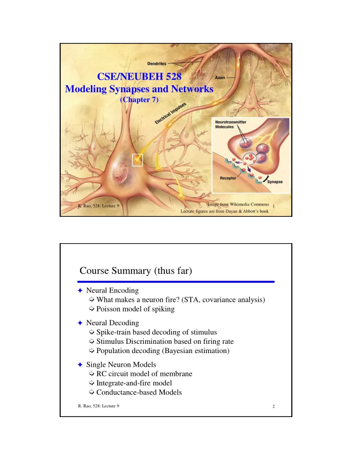
CSE/NEUBEH 528 Modeling Synapses and Networks

(Chapter 7)

Image from Wikimedia Commons

Lecture figures are from Dayan & Abbott’s book 2

• R. Rao, 528: Lecture 9

Course Summary (thus far)

F Neural Encoding

What makes a neuron fire? (STA, covariance analysis) Poisson model of spiking

F Neural Decoding

Spike-train based decoding of stimulus Stimulus Discrimination based on firing rate Population decoding (Bayesian estimation)

F Single Neuron Models

RC circuit model of membrane Integrate-and-fire model Conductance-based Models

3

• R. Rao, 528: Lecture 9

Today’s Agenda

F Computation in Networks of Neurons

Modeling synaptic inputs From spiking to firing-rate based networks Feedforward Networks Linear Recurrent Networks

4

• R. Rao, 528: Lecture 9

SYNAPSES!

Image Credit: Kennedy lab, Caltech. http://www.its.caltech.edu/~mbkla

5

• R. Rao, 528: Lecture 9

What do synapses do?

Increase or decrease postsynaptic membrane potential Spike

Image Source: Wikimedia Commons 6

• R. Rao, 528: Lecture 9

An Excitatory Synapse

Input spike  Neurotransmitter release (e.g., Glutamate)  Binds to receptors  Ion channels open  positive ions (e.g. Na+) enter cell  Depolarization due to EPSP (excitatory postsynaptic potential)

Image Source: Wikimedia Commons

Spike

7

• R. Rao, 528: Lecture 9

An Inhibitory Synapse

Input spike  Neurotransmitter release (e.g., GABA)

 Binds to receptors

 Ion channels open

 positive ions (e.g.,

K+) leave cell  Hyperpolarization due to IPSP (inhibitory postsynaptic potential)

Image Source: Wikimedia Commons

Spike

8

• R. Rao, 528: Lecture 9

Flashback Membrane Model

ly equivalent

• r

, ) ( A I r E V dt dV c

e m L m

   

m e L m

R I E V dt dV     ) ( 

m = rmcm= RmCm membrane time constant

V

9

• R. Rao, 528: Lecture 9

Flashback! The Integrate-and-Fire Model

V

m e L m

R I E V dt dV     ) ( 

mV 70  

L

E

If V > Vthreshold  Spike Then reset: V = Vreset

(resting potential)

mV 50  

threshold

V

L reset

E V 

Models a passive leaky membrane

10

• R. Rao, 528: Lecture 9

Flashback! Hodgkin-Huxley Model

) ( ) ( ) (

3 max , 4 max , max , Na Na K K L L m e m m

E V h m g E V n g E V g i A I i dt dV c         

EL = -54 mV, EK = -77 mV, ENa = +50 mV L K Na

11

• R. Rao, 528: Lecture 9

How do we model the effects of a synapse on the membrane potential V ?

Synapse

?

12

• R. Rao, 528: Lecture 9

V

s rel s s m e s s m L m

P P g g R I E V g r E V dt dV

max ,

) ( ) (        

Probability of transmitter release given an input spike Probability of postsynaptic channel opening (= fraction of channels opened)

Synaptic conductance

Modeling Synaptic Inputs

Synapse

13

• R. Rao, 528: Lecture 9

Basic Synapse Model

F Assume Prel = 1 F Model the effect of a single spike input on Ps F Kinetic Model of postsynaptic channels:

s s s s s

P P dt dP      ) 1 (

   

s s

 

Opening rate Closing rate Fraction of channels closed Fraction of channels open Closed Open fraction of channels

• pened

14

• R. Rao, 528: Lecture 9

What does Ps look like over time?

Exponential function K(t) gives reasonable fit to biological data (other options: difference of exponentials, “alpha” function)

s

t s

e t K







 1 ) (

15

• R. Rao, 528: Lecture 9

Linear Filter Model of Synaptic Input to a Neuron

    d t K w t t K w t I

t b b t t i b b

i

) ( ) ( ) ( ) (

 

  

   

Synaptic current for b: b(t) = i δ(t-ti) (ti are the input spike times) Filter for synapse b:

s

t s

e t K







 1 ) (

wb

Input Spike Train b(t) Synaptic weight

16

• R. Rao, 528: Lecture 9

Modeling Networks of Neurons

F Option 1: Use spiking neurons Advantages: Model computation and learning based on: Spike Timing Spike Correlations/Synchrony between neurons Disadvantages: Computationally expensive F Option 2: Use neurons with firing-rate outputs (real

valued outputs)

Advantages: Greater efficiency, scales well to large networks Disadvantages: Ignores spike timing issues F Question: How are these two approaches related?

17

• R. Rao, 528: Lecture 9

From Spiking to Firing Rate Models

wN Firing rate ub(t)

Spikes 1(t)

   

   

   

b t b b b t b b s

d u t K w d t K w t I        ) ( ) ( ) ( ) ( ) (

) ( ) ( t I t I

b b s





Total synaptic current

Spike train b(t) w1

Spikes N(t)

18

• R. Rao, 528: Lecture 9

Synaptic Current Dynamics in Firing Rate Model

F Suppose synaptic kernel K is exponential:

Differentiating w.r.t. time t, we get

 

 

 

b t b b s

d u t K w t I    ) ( ) ( ) (

u w      



s b b b s s s

I u w I dt dI 

s

t s

e t K







 1 ) (

19

• R. Rao, 528: Lecture 9

Output Firing-Rate Dynamics

F How is the output firing rate v related to synaptic inputs? F Looks very much like membrane equation: F On-board derivations of special cases obtained from

comparing the relative magnitudes of r and s … (see also pages 234-236 in the text)

)) ( ( t I F v dt dv

s r

   

m e L m

R I E V dt dV     ) (  u w    

s s s

I dt dI 

20

• R. Rao, 528: Lecture 9

How good are Firing Rate Models?

Firing rate model v(t) = F(I(t)) describes this well but not this case Input I(t) = I0 + I1cos(t)

21

• R. Rao, 528: Lecture 9

Feedforward versus Recurrent Networks

) M W ( v u v v     F dt d 

For feedforward networks, matrix M = 0

Output Decay Input Feedback

22

• R. Rao, 528: Lecture 9

Example: Linear Feedforward Network

u v v W    dt d  Dynamics: Steady State

(set dv/dt to 0):

u v W 

ss

                                            1 2 2 2 1 1 1 1 1 1 1 1 1 1 1 1 1 W u

What is vss?

23

• R. Rao, 528: Lecture 9

Linear Feedforward Network

                                                                  1 1 1 2 2 2 1 1 1 1 1 1 1 1 1 1 1 1 1 Wu vss

What is the network doing?

24

• R. Rao, 528: Lecture 9

Linear Filtering for Edge Detection

 

                                       1 1 Output 1 2 2 2 1 Input W) in versions shifted (and 1 1 Filter Input Output

25

• R. Rao, 528: Lecture 9

Example of Edge Detection in a 2D Image

http://www.alexandria.nu/ai/blog/entry.asp?E=51

26

• R. Rao, 528: Lecture 9

Edge detectors in the visual system

Examples of receptive fields in primary visual cortex (V1)

V1

(From Nicholls et al., 1992)

27

• R. Rao, 528: Lecture 9

Filtering network is computing derivatives!

) ( ) 1 ( ion approximat Discrete ) ( ) ( lim x f x f h x f h x f dx df

h

     



   

) 1 ( ) ( 2 ) 1 ( ) 1 ( ) ( ) ( ) 1 ( approx. Disc. ) ( ) ( lim

2 2

               



x f x f x f x f x f x f x f h x f h x f dx f d

h

 

1 1 

 

1 2 1 

28

• R. Rao, 528: Lecture 9

Feedforward Networks: Example 2

Input: Area 7a Neurons with Gaze-Dependent Tuning Curves Output: Premotor Cortex Neuron with Body-Based Tuning Curves

Coordinate Transformation

(From Section 7.3 in Dayan & Abbott)

29

• R. Rao, 528: Lecture 9

Output of Coordinate Transformation Network

Same tuning curve regardless of gaze angle

Premotor cortex neuron responds to stimulus location relative to body, not retinal image location Head fixed; gaze shifted to g1 g2 g3 (See section 7.3 in Dayan & Abbott for details)

30

• R. Rao, 528: Lecture 9

Linear Recurrent Networks

v u v v M W     dt d 

Output Decay Input Feedback

31

• R. Rao, 528: Lecture 9

Next Class: Recurrent Networks

F To Do:

Homework 2 Find a final project topic and partner(s)