Lecture 13: From Unsupervised to Reinforcement Learning (Chapters - PDF document

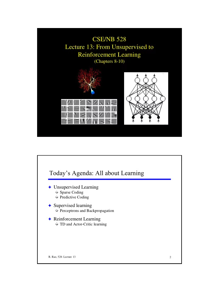
CSE/NB 528 Lecture 13: From Unsupervised to Reinforcement Learning (Chapters 8-10) R. Rao, 528: Lecture 13 1 Today’s Agenda: All about Learning F Unsupervised Learning Sparse Coding Predictive Coding F Supervised learning Perceptrons and Backpropagation F Reinforcement Learning TD and Actor-Critic learning R. Rao, 528: Lecture 13 2

Recall from Last Time: Linear Generative Model Suppose input u was Causes v generated by a linear superposition of causes v 1 , v 2 , …, v k with basis Generative vectors (or “features”) g i model      u g v v noise G n i i i Data u (Assume noise is Gaussian white noise with mean zero) R. Rao, 528: Lecture 13 3 Bayesian approach F Find v and G that maximize posterior:   [ | ; ] [ | ; ] [ ; ] p v u G k p u v G p v G F Equivalently, find v and G that maximize log posterior:    ( , ) log [ | ; ] log [ ; ] log F v G p u v G p v G k  G  u v n If v a independent log of Gaussian   p [ v ; G ] p [ v ; G ] a log ( ; , ) N u G v I a   1 log p [ v ; G ] log p [ v ; G ]      T a ( u G v ) ( u G v ) C a 2 Prior for individual causes (what R. Rao, 528: Lecture 13 4 should this be?)

What do we know about the causes v ? F Idea: Causes independent: only a few of them will be active for any input v a will be 0 most of the time but high for a few inputs Suggests a sparse distribution for p [ v a ; G ]: peak at 0 but with heavy tail (also called super-Gaussian distribution) R. Rao, 528: Lecture 13 5 Examples of Prior Distributions for Causes Possible prior Log prior distributions   ( ) | | g v v sparse    2 g ( v ) log( 1 v )    p [ v ; G ] c exp( g ( v )) a a    log [ ; ] ( ) p v G g v c a a R. Rao, 528: Lecture 13 6

Finding the optimal v and G F Want to maximize:    ( , ) log [ | ; ] log [ ; ] log F v G p u v G p v G k 1        T ( ) ( ) ( ) u G v u G v g v K a 2 a F Alternate between two steps: Maximize F with respect to v keeping G fixed How? Maximize F with respect to G, given the v above How? R. Rao, 528: Lecture 13 7 Estimating the causes v for a given input Derivative of g Gradient d v dF      T ( ) ( ) G u G v g v ascent dt d v Reconstruction (prediction) of u v d  Firing rate dynamics     T ( ) ( ) G u G v g v (Recurrent network) dt Error Sparseness constraint R. Rao, 528: Lecture 13 8

Sparse Coding Network for Estimating v d v      T ( ) ( ) G u G v g v dt Corrected Estimate  ( ) G v u G v Prediction Error [Suggests a role for feedback pathways in the cortex (Rao & Ballard, 1999) ] R. Rao, 528: Lecture 13 9 Learning the Synaptic Weights G  ( ) G v u G v Prediction Error dG dF Gradient   (  T ) u G v v ascent dt dG dG Learning Hebbian!   (  T ) u G v v (similar to Oja’s rule) rule G dt R. Rao, 528: Lecture 13 10

Result: Learning G for Natural Images Each square is a column g i of G (obtained by collapsing rows of the square into a vector) Almost all the g i represent local edge features Any image patch u can be expressed as:    u g v G v i i i (Olshausen & Field, 1996) R. Rao, 528: Lecture 13 11 Sparse Coding Network is a special case of Predictive Coding Networks (Rao, Vision Research , 1999) R. Rao, 528: Lecture 13 12

Predictive Coding Model of Visual Cortex (Rao & Ballard, Nature Neurosci ., 1999) R. Rao, 528: Lecture 13 13 Predictive coding model explains contextual effects Monkey Primary Visual Cortex Model (Zipser et al., J. Neurosci ., 1996) Increased activity for non-homogenous input interpreted as prediction error (i.e., anomalous input): center is not predicted by surrounding context. R. Rao, 528: Lecture 13 14

Natural Images as a Source of Contextual Effects Center predictable from Surround R. Rao, 528: Lecture 13 15 (Rao & Ballard, Nature Neurosci ., 1999) What if your data comes with not just inputs but also outputs? Enter…Supervised Learning R. Rao, 528: Lecture 13 16

Supervised Learning F Two Primary Tasks 1. Classification Inputs u 1 , u 2 , … and discrete classes C 1 , C 2 , …, C k Training examples: (u 1 , C 2 ), (u 2 , C 7 ), etc. Learn the mapping from an arbitrary input to its class Example: Inputs = images, output classes = face, not a face 2. Regression Inputs u 1 , u 2 , … and continuous outputs v 1 , v 2 , … Training examples: (input, desired output) pairs Learn to map an arbitrary input to its corresponding output Example: Highway driving Input = road image, output = steering angle R. Rao, 528: Lecture 13 17 The Classification Problem denotes output of +1 (faces) Faces denotes output of -1 (other) Other objects Idea: Find a separating hyperplane (line in this case) R. Rao, 528: Lecture 13 18

Neurons as Classifiers: The “Perceptron” F Artificial neuron: m binary inputs (-1 or 1) and 1 output (-1 or 1)  Synaptic weights w ij     ( ) v w u Threshold  i i ij j i j  (x) = +1 if x  0 and -1 if x < 0 Weighted Sum Threshold Inputs u j Output v i (-1 or +1) (-1 or +1) R. Rao, 528: Lecture 13 19 What does a Perceptron compute? F Consider a single-layer perceptron Weighted sum forms a linear hyperplane (line, plane, …)     0 w ij u j i j Everything on one side of hyperplane is in class 1 (output = +1) and everything on other side is class 2 (output = -1) Any function that is linearly separable can be computed by a perceptron R. Rao, 528: Lecture 13 20

Linear Separability F Example: AND function is linearly separable a AND b = 1 if and only if a = 1 and b = 1 u 2 (1,1) v Linear hyperplane  = 1.5 1 u 1 -1 1 u 1 u 2 -1 +1 output Perceptron for AND -1 output R. Rao, 528: Lecture 13 21 What about the XOR function? ? u 1 u 2 XOR +1 output u 2 -1 output -1 -1 +1 1 1 -1 -1 1 u 1 -1 1 -1 -1 1 1 +1 -1 Can a straight line separate the +1 outputs from the -1 outputs? R. Rao, 528: Lecture 13 22

Multilayer Perceptrons F Removes limitations of single-layer networks Can solve XOR F An example of a two-layer perceptron that computes XOR  = -1 1 1 2  = 1.5 -1 -1 y x F Output is +1 if and only if x + y + 2  ( – x – y – 1.5) > – 1 (Inputs x and y can be +1 or -1) R. Rao, 528: Lecture 13 23 What if you want to approximate a continuous function (i.e., regression)? Can a network learn to drive? R. Rao, 528: Lecture 13 24

Example Network Steering angle Desired Output: d = [d 1 d 2 … d 30 ] Current image Input u = [u 1 u 2 … u 960 ] = image pixels R. Rao, 528: Lecture 13 25 Sigmoid Networks    T ( ) ( ) Sigmoid output function: v g w u g w u Output i i 1 i  1 ( ) g a    a e w g(a)  (a) Input nodes 1 u = (u 1 u 2 u 3 ) T a Sigmoid is a non- linear “squashing” function: Squashes input to be between 0 and 1. Parameter  controls the slope. R. Rao, 528: Lecture 13 26

Multilayer Sigmoid Networks    v g ( W g ( w u )) i ji kj k j k Output v = (v 1 v 2 … v J ) T ; Desired = d How do we learn these weights? Input u = (u 1 u 2 … u K ) T R. Rao, 528: Lecture 13 27 Backpropagation Learning: Uppermost layer   v g ( W x ) i ji j Minimize output error: j   1  2 ( , ) ( ) E W w d v i i 2 i x j u k Learning rule for hidden-output weights W : dE    W W { gradient descent } ji ji dW ji dE      ( ) ( ) d v g W x x { delta rule } i i ji j j dW j ji R. Rao, 528: Lecture 13 28

Backpropagation: Inner layer (chain rule)   m v g ( W x ) Minimize output error: i ji j j   1  2 ( , ) ( ) E W w d v i i  2  m m i ( ) x g w u j kj k k m u k Learning rule for input-hidden weights w : dx dE dE dE      j But : w w { chain rule } kj kj dw dw dx dw kj kj j kj      dE         m m m m m  ( ) ( )  ( ) d v g W x W  g w u u  i i ji j ji kj k k   dw   , m i j k kj R. Rao, 528: Lecture 13 29 Demos: Pole Balancing and Backing up a Truck (courtesy of Keith Grochow, CSE 599) v pole • Neural network learns to balance a pole on a cart • System : x cart • 4 state variables: x cart , v cart , θ pole , v pole θ pole • 1 input: Force on cart • Backprop Network: v cart • Input: State variables • Output: New force on cart • NN learns to back a truck into a loading dock • System (Nyugen and Widrow, 1989): • State variables: x cab , y cab , θ cab • 1 input: new θ steering • Backprop Network: • Input: State variables • Output: Steering angle θ steering R. Rao, 528: Lecture 13 30