
SLIDE 1
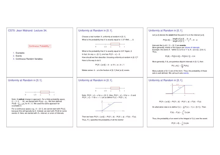
CS70: Jean Walrand: Lecture 34.
Continuous Probability 1
- 1. Examples
- 2. Events
- 3. Continuous Random Variables
Uniformly at Random in [0,1].
Choose a real number X, uniformly at random in [0,1]. What is the probability that X is exactly equal to 1/3? Well, ..., 0. What is the probability that X is exactly equal to 0.6? Again, 0. In fact, for any x ∈ [0,1], one has Pr[X = x] = 0. How should we then describe ‘choosing uniformly at random in [0,1]’? Here is the way to do it: Pr[X ∈ [a,b]] = b −a,∀0 ≤ a ≤ b ≤ 1. Makes sense: b −a is the fraction of [0,1] that [a,b] covers.
Uniformly at Random in [0,1].
Let [a,b] denote the event that the point X is in the interval [a,b]. Pr[[a,b]] = length of [a,b] length of [0,1] = b −a 1 = b −a. Intervals like [a,b] ⊆ Ω = [0,1] are events. More generally, events in this space are unions of intervals. Example: the event A - “within 0.2 of 0 or 1” is A = [0,0.2]∪[0.8,1]. Thus, Pr[A] = Pr[[0,0.2]]+Pr[[0.8,1]] = 0.4. More generally, if An are pairwise disjoint intervals in [0,1], then Pr[∪nAn] := ∑
n
Pr[An]. Many subsets of [0,1] are of this form. Thus, the probability of those sets is well defined. We call such sets events.
Uniformly at Random in [0,1].
Note: A radical change in approach. For a finite probability space, Ω = {1,2,...,N}, we started with Pr[ω] = pω. We then defined Pr[A] = ∑ω∈A pω for A ⊂ Ω. We used the same approach for countable Ω. For a continuous space, e.g., Ω = [0,1], we cannot start with Pr[ω], because this will typically be 0. Instead, we start with Pr[A] for some events A. Here, we started with A = interval, or union of intervals.
Uniformly at Random in [0,1].
Note: Pr[X ≤ x] = x for x ∈ [0,1]. Also, Pr[X ≤ x] = 0 for x < 0 and Pr[X ≤ x] = 1 for x > 1. Let us define F(x) = Pr[X ≤ x]. Then we have Pr[X ∈ (a,b]] = Pr[X ≤ b]−Pr[X ≤ a] = F(b)−F(a). Thus, F(·) specifies the probability of all the events!
Uniformly at Random in [0,1].
Pr[X ∈ (a,b]] = Pr[X ≤ b]−Pr[X ≤ a] = F(b)−F(a). An alternative view is to define f(x) = d
dx F(x) = 1{x ∈ [0,1]}. Then
F(b)−F(a) =
b
a f(x)dx.
Thus, the probability of an event is the integral of f(x) over the event: Pr[X ∈ A] =
- A f(x)dx.