SLIDE 1
CS302 Topic: Algorithm Analysis
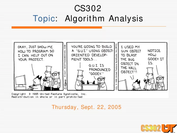
Thursday, Sept. 22, 2005
SLIDE 2 Announcements
- Lab 3 (Stock Charts with graphical objects) is due this
Friday, Sept. 23!!
- Lab 4 now available (Stock Reports); due Friday, Oct. 7
(2 weeks)
Don’t procrastinate!! Procrastination is like a credit card: Procrastination is like a credit card: it’s a lot of fun until you get the bill. it’s a lot of fun until you get the bill.
Christopher Parker
SLIDE 3 Check your knowledge of C+ + & libs:
Assume:
- a. Stack()
- b. Stack(int size);
- c. Stack(const Stack &);
- d. Stack &operator= (const Stack &)
Which type of constructor gets called?
b
Answer:
Stack *stack1 = new Stack(10);
#8
SLIDE 4 Check your knowledge of C+ + & libs:
Assume:
- a. Stack()
- b. Stack(int size);
- c. Stack(const Stack &);
- d. Stack &operator= (const Stack &)
Which type of constructor gets called?
a
Answer:
Stack stack2;
#9
SLIDE 5 Check your knowledge of C+ + & libs:
Assume:
- a. Stack()
- b. Stack(int size);
- c. Stack(const Stack &);
- d. Stack &operator= (const Stack &)
Which type of constructor gets called?
c
Answer:
Stack stack3 = stack2;
#10
SLIDE 6 Check your knowledge of C+ + & libs:
Assume:
- a. Stack()
- b. Stack(int size);
- c. Stack(const Stack &);
- d. Stack &operator= (const Stack &)
Which type of constructor gets called?
c
Answer:
Stack stack4(stack2);
#11
SLIDE 7 Check your knowledge of C+ + & libs:
Assume:
- a. Stack()
- b. Stack(int size);
- c. Stack(const Stack &);
- d. Stack &operator = (const Stack &)
Which type of constructor gets called?
d
Answer:
stack4 = stack2;
#12
SLIDE 8 Analysis of Algorithms
- The theoretical study of computer program performance and
resource usage
- What’s also important (besides performance/ resource usage)?
- Modularity
- Correctness
- Maintainability
- Functionality
- Robustness
- User-friendliness
- Programmer time
- Simplicity
- Reliability
SLIDE 9
Why study algorithms and performance?
Analysis helps us understand scalability Performance often draws the line between what is feasible and what is impossible Algorithmic mathematics provides a language for talking about program behavior The lessons of program performance generalize to other computing resources Speed is fun!
SLIDE 10 The problem of sorting
Input: sequence
Output: permutation such that Example:
8 2 4 9 3 6
2 3 4 6 8 9
1 2
, ,...,
n
a a a < >
1 2
, ,...,
n
a a a ′ ′ ′ < >
1 2
...
n
a a a ′ ′ ′ ≤ ≤ ≤
SLIDE 11 Insertion sort
I NSERTION-SORT(A,n) A[ 1 .. n] for j ← 2 to n do key ← A[ j] i ← j – 1 while i > 0 and A[ i] > key do A[ i + 1] ← A[ i] i ← i – 1 A[ i + 1] = key
“pseudocode” 1 i j n
key
sorted
A:
SLIDE 12 Example of insertion sort
8 2 4 9 3 6 2 8 4 9 3 6 2 4 8 9 3 6 2 4 8 9 3 6 2 3 4 8 9 6 2 3 4 6 8 9
done
SLIDE 13
Running time
Running time depends on the input; an already-sorted sequence is easier to sort Parameterize the running time by the size of the input, since short sequences are easier to sort than long ones Generally, we seek an upper bounds on the running time, since everybody likes a guarantee
SLIDE 14 Kinds of analyses
Worst-case: (usually)
- T(n) = maximum time of algorithm on any input
- f size n
Average case: (sometimes)
- T(n) = expected time of algorithm over all
inputs of size n
- Need assumption of statistical distribution of
inputs
Best case: (bogus)
- Cheat with a slow algorithm that works fast on
some input
SLIDE 15 Machine-independent time
What is insertion sort’s worst-case time?
- It depends on the speed of our computer
- Relative speed (on the same machine)
- Absolute speed (on different machines)
- B
BI G
I G I
I DEA
DEA:
:
- Ignore machine-dependent constants
- Look at growth of T(n) as n → ∞
“Asymptotic Analysis” “Asymptotic Analysis”
SLIDE 16 Θ-notation (tight upper bound)
Θ(n2): Pronounce it: “Theta of n2” Math: Θ(g(n)) = { f(n):
there exist positive constants c1, c2, and n0, such that 0 ≤ c1 g(n) ≤ f(n) ≤ c2 g(n) for all n ≥ n0 }
Engineering:
- Drop low-order terms; ignore leading constants
- Example:
3n3 + 90n2 – 4n + 6046 = Θ(n3)
SLIDE 17 Asymptotic performance
When n gets large enough, a Θ(n2) algorithm always beats a Θ(n3) algorithm
asymptotically slower algorithms, however.
- real-world design situations
- ften call for a careful
balancing of engineering
- bjectives
- Asymptotic analysis is a
useful tool to help structure
SLIDE 18
Closer look at mathematical definition of Θ(n)
Θ(g(n)) = { f(n):
there exist positive constants c1, c2, and n0, such that 0 ≤ c1 g(n) ≤ f(n) ≤ c2 g(n) for all n ≥ n0 }
f(n) c2g(n) c1g(n) n0 n f(n) = Θ(g(n))
SLIDE 19
O-notation (upper bound – may
not be tight upper bound)
O(n2): Pronounce it: “Big-Oh of n2” or “Order n2” Math:
O(g(n)) = { f(n): there exist positive constants c and n0, such that 0 ≤ f(n) ≤ cg(n) for all n ≥ n0 }
SLIDE 20
Closer look at mathematical definition of O(n)
O(g(n)) = { f(n): there exist positive constants c and n0, such that 0 ≤ f(n) ≤ cg(n) for all n ≥ n0 }
f(n) cg(n) n0 n f(n) = O(g(n))
SLIDE 21 Insertion sort analysis
Input reverse sorted
All permutations equally likely
- Is insertion sort a fast sorting algorithm?
- Moderately so, for small n
- Not at all, for large n
2 2
( ) ( ) ( )
n j
T n j n
=
= Θ = Θ
∑
[ Recall arithmetic series: ]
2 1 2 1
( 1) ( )
n k
k n n n
=
= + = Θ
∑
2 2
( ) ( / 2) ( )
n j
T n j n
=
= Θ = Θ
∑
SLIDE 22 Merge sort
MERGE-SORT A[ 1..n]
- 1. If n = 1, we’re done.
- 2. Recursively sort A[ 1..⎡n/ 2⎤ ] and A[ ⎡n/ 2⎤+ 1 .. n ]
- 3. “Merge” the 2 sorted arrays
Subroutine MERGE
- From the head of each array, output the smallest
value and increment the pointer to that array; continue until reach end of both arrays
SLIDE 23
Merging two sorted arrays
20 12 13 11 7 9 2 1 1
SLIDE 24
Merging two sorted arrays
20 12 13 11 7 9 2 1 1 20 12 13 11 7 9 2 2
SLIDE 25
Merging two sorted arrays
20 12 13 11 7 9 2 1 1 20 12 13 11 7 9 2 2 20 12 13 11 7 9 7
SLIDE 26
Merging two sorted arrays
20 12 13 11 7 9 2 1 1 20 12 13 11 7 9 2 2 20 12 13 11 7 9 7 20 12 13 11 9 9
SLIDE 27 Merging two sorted arrays
20 12 13 11 7 9 2 1 1 20 12 13 11 7 9 2 2 20 12 13 11 7 9 7 20 12 13 11 9 9 20 12 13 11 11
Etc.
Time = Θ(n) to merge a total
- f n elements (i.e., linear time)
SLIDE 28
Analyzing merge sort
T(n) Θ(1)
2 T(n/ 2)
Θ(n) MERGE-SORT A[ 1..n]
1.If n = 1, we’re done. 2.Recursively sort A[ 1..⎡n/ 2⎤ ] and A[ ⎡n/ 2⎤+ 1 .. n ] 3.“Merge” the 2 sorted arrays Sloppiness: turns out not to matter asymptotically Should be T[ ⎡n/ 2⎤ ] + T[ ⎣n/ 2⎦ ] , but it Means constant time
SLIDE 29
Recurrence for merge sort
Recurrence: an equation defined in terms of itself For merge sort: We usually omit stating the base case when T(n) = Θ(1) for sufficiently small n, but only when it has no effect on the asymptotic solution to the recurrence
(1) if 1 ( ) 2 ( / 2) ( ) if 1 n T n T n n n Θ = ⎧ = ⎨ + Θ > ⎩
SLIDE 30
Solving recurrences: The recursion tree
Solve T(n) = 2T(n/ 2) + cn, for constant c > 0 T(n)
SLIDE 31
Solving recurrences: The recursion tree
Solve T(n) = 2T(n/ 2) + cn, for constant c > 0 cn T(n/ 2) T(n/ 2)
SLIDE 32
Solving recurrences: The recursion tree
Solve T(n) = 2T(n/ 2) + cn, for constant c > 0 cn T(n/ 4) T(n/ 4) cn/ 2 cn/ 2 T(n/ 4) T(n/ 4)
SLIDE 33
Solving recurrences: The recursion tree
Solve T(n) = 2T(n/ 2) + cn, for constant c > 0 cn cn/ 4 cn/ 4 cn/ 2 cn/ 2 cn/ 4 cn/ 4
…
Θ(1)
SLIDE 34
Solving recurrences: The recursion tree
Solve T(n) = 2T(n/ 2) + cn, for constant c > 0 cn cn/ 4 cn/ 4 cn/ 2 cn/ 2 cn/ 4 cn/ 4
…
Θ(1) h = lg n
SLIDE 35
Solving recurrences: The recursion tree
Solve T(n) = 2T(n/ 2) + cn, for constant c > 0 cn cn/ 4 cn/ 4 cn/ 2 cn/ 2 cn/ 4 cn cn/ 4
…
Θ(1) h = lg n
SLIDE 36
Solving recurrences: The recursion tree
Solve T(n) = 2T(n/ 2) + cn, for constant c > 0 cn cn/ 4 cn/ 4 cn/ 2 cn/ 2 cn/ 4 cn cn/ 4
…
Θ(1) h = lg n cn
SLIDE 37
Solving recurrences: The recursion tree
Solve T(n) = 2T(n/ 2) + cn, for constant c > 0 cn cn/ 4 cn/ 4 cn/ 2 cn/ 2 cn/ 4 cn cn/ 4
…
Θ(1) h = lg n cn cn
…
SLIDE 38 Solving recurrences: The recursion tree
Solve T(n) = 2T(n/ 2) + cn, for constant c > 0 cn cn/ 4 cn/ 4 cn/ 2 cn/ 2 cn/ 4 cn cn/ 4
…
Θ(1) h = lg n cn cn
…
# leaves = n
Θ(n)
SLIDE 39 Solving recurrences: The recursion tree
Solve T(n) = 2T(n/ 2) + cn, for constant c > 0 cn cn/ 4 cn/ 4 cn/ 2 cn/ 2 cn/ 4 cn cn/ 4
…
cn cn Θ(1) Θ(n)
# leaves = n
h = lg n
…
SLIDE 40 Solving recurrences: The recursion tree
Solve T(n) = 2T(n/ 2) + cn, for constant c > 0 cn cn/ 4 cn/ 4 cn/ 2 cn/ 2 cn/ 4 cn cn/ 4
…
cn cn Θ(1) Θ(n)
# leaves = n
h = lg n
…
SLIDE 41 Solving recurrences: The recursion tree
Solve T(n) = 2T(n/ 2) + cn, for constant c > 0 cn cn/ 4 cn/ 4 cn/ 2 cn/ 2 cn/ 4 cn cn/ 4
…
Θ(1) cn cn Θ(n)
# leaves = n
h = lg n
…
Total = Θ(n lg n)
SLIDE 42
Differences in asymptotic complexity
Θ(n lg n) grows more slowly than Θ(n2) Therefore, merge sort asymptotically beats insertion sort in the worst case In practice, merge sort beats insertion sort for n > 30 (or so)
SLIDE 43
To get a feel for differences in run time, watch this animation
Compare Θ(n2) algorithm with Θ(n log n) (and algorithms run on sequential versus parallel machines): http: / / www.cs.rit.edu/ ~ atk/ Java/ Sorting/ sorting.html
SLIDE 44 Options for solving recurrences
Recursion tree Proof by induction (beyond scope of this class) Master method (beyond scope of this class)
- Solves recurrences of the form:
Learn common solutions, such as:
( ) ( / ) ( ) T n aT n b f n = +
Recurrence: ( ) ( / 2) ( ) ( / 2) ( ) 2 ( / 2) ( ) 2 ( / 2) ( ) ( 1) T n T n d T n T n n T n T n d T n T n n T n T n d = + = + = + = + = − + Solution: ( ) (log ) ( ) ( ) ( ) ( ) ( ) ( log ) ( ) ( ) T n O n T n O n T n O n T n O n n T n O n = = = = =
SLIDE 45 Typical running times of algorithms
Θ(1): The running time of the program is constant (i.e., independent of the size of the input)
Find the 5th element in an array
Θ(log n): Typically achieved by dividing the problem into smaller segments and only looking at one input element in each segment
Θ(n): Typically achieved by examining each input element once
Find the minimum element
SLIDE 46 Typical running times of algorithms (con’t.)
Θ(n log n): Typically achieved by dividing the problem into subproblems, solving the subproblems independently, and then combining the results. Here, each element in subproblem must be examined.
Merge sort
Θ(n2): Typically achieved by examining all pairs of data elements
Insertion sort
Θ(n3): Often achieved by combining algorithms with a mixture of the previous running times
Matrix Multiplication
SLIDE 47
That’s all, folks.
Questions?